We have discussed several aspects of deep learning theory, ranging from optimization and generalization guarantees to role of depth and generative models. In this final post of this series, I will illustrate how theory can motivate simple solutions to problems, which can then outperform complex techniques. For this, we will consider a field where deep learning has done exceptionally well, namely, word and sentence embeddings.
If you need a refresher on word embeddings, I have previously explained them, along with the most popular methods, in this post. The distributional hypothesis forms the basis for all word embedding techniques used at present. Instead of naively taking the co-occurence matrix, though, almost all techniques use some low-rank approximation for the same. This gives rise to low-dimensional ($\sim 300$) dense embeddings for text. An important question, then, is the following: How can low-dimensional embeddings represent the complex linguistic structure in text? We will first look at this question from a theoretical perspective, based on this ACL’16 paper from Arora et al.
How do low-dimensional embeddings approximate co-occurence matrices?
Formally, we want to see why, for some low-dimensional vector representations $v$, we have
\[\langle v_w,v_{w^{\prime}} \rangle \approx \text{PMI}(w,w^{\prime}),\]where $\text{PMI}(w,w^{\prime})$ is the pointwise mutual information between $w$ and $w^{\prime}$, defined as $\log \frac{P(w,w^{\prime})}{P(w)P(w^{\prime})}$, where the probabilities are computed empirically from the co-occurence matrix.
For this, the authors propose a generative model of language, as opposed to the usual discriminative model that is based on predicting the context words given a target word (i.e., multiclass classification). This is based on the random walk of a discourse vector $c_t \in \mathcal{R}^d$, which generates $t$th word in step $t$. Every word has a time-invariant latent vector $v_w \in \mathcal{R}^d$, and the word production model is given as
\[\text{Pr}[w ~ \text{emitted at time} ~ t|c_t] \propto \exp(\langle c_t,v_w \rangle).\]Here, random walk means that $c_{t+1}$ is obtained by adding a small random displacement vector to $c_t$. For a theoretic analysis, we make an isotropy assumption about the word vectors.
Isotropy assumption: In the bulk, word vectors are distributed uniformly in the $\mathcal{R}^d$ space.
To generate such a dsitribution, we can just sample i.i.d from $v = s \cdot v^{\prime}$, where $s$ is a scalar random variable ($s \leq \kappa$), and $v^{\prime}$ is obtained from a spherical Gaussian distribution. This is a simple Bayesian prior similar to the assumptions commonly used in statistics.
Let us define $Z_c = \sum_{w}\exp(\langle v_w,c \rangle)$. This is like the normalization factor used with the above equation, but it is very difficult to compute. In the paper, the authors prove that this value is very close to some constant $Z$ for a fixed $c$. This allows us to remove this factor from consideration. Empirically, it has also been seen that some log-linear models have self-normalization properties, and this may be a reason for the observation. Let us now see how to prove this lemma.
Since $Z_c$ is a sum of random variables, it may be tempting to use concentration inequalities to bound its value. However, we cannot do this since $Z_c$ is neither sub-Gaussian nor sub-exponential. We approach the problem it two parts. First we bound the mean and variance of $Z_c$, and then show that it is concentrated around its mean.
Part 1: Suppose there are $n$ vectors in our space. Since they are identically distributed, we have
\[\mathbb{E}[Z_c] = n\mathbb{E}[\exp(\langle v_w,c \rangle)] \geq n\mathbb{E}[1 + \langle v_w,c \rangle] = n.\]Here, we have used $\mathbb{E}[\langle v_w,c \rangle] = 0$, since $v_w$’s are drawn from a scaled uniform spherical Gaussian. Now, suppose all the scalar variables $s_w$ are equal in distribution to $s$. Then, we can write
\[\mathbb{E}[Z_c] = n\mathbb{E}[\exp(\langle v_w,c \rangle)] = n\mathbb{E}\left[ \mathbb{E} [\exp(\langle v_w,c \rangle)|s]\right].\]We can compute the conditional expectation as
\[\begin{align} \mathbb{E} [\exp(\langle v_w,c \rangle)|s] &= \int_x \frac{1}{\sigma\sqrt{2\pi}}\exp\left( -\frac{x^2}{2\sigma^2} \right)\exp(x) dx \\ &= \frac{1}{\sigma\sqrt{2\pi}}\exp\left( -\frac{(x-\sigma^2)^2}{2\sigma^2} + \frac{\sigma^2}{2}\right) dx \\ &= \exp(\frac{\sigma^2}{2}). \end{align}\]Here, the standard deviation is equal to the scaling factor $s$, and so $\sigma^2 = s^2$. It follows that
\[\mathbb{E}(Z_c) = n\exp(\frac{s^2}{2}).\]Similarly, we can show that the variance
\[\mathbb{V}(Z_c) \leq n\mathbb{E}[\exp(2s^2)].\]Since $\langle v_w,c \rangle\vert s$ has a Gaussian distribution with variance $s^2 \leq \kappa^2$, we have using Chernoff bounds that
\[\text{Pr}[|\langle v_w,c \rangle| \geq \eta \log n |s] \leq \exp \left( - \frac{\eta^2 \log^2 n}{2\kappa^2} \right) = \exp (-\Omega(\log^2 n)).\]Here we have removed $\eta$ and $\kappa$ since they are constants. We can now write the converse of this inequality, by taking expectation over all $s_w$, as
\[\text{Pr}[|\langle v_w,c \rangle| \leq \frac{1}{2}\log n] \geq 1 - \exp(-\Omega(\log^2 n)).\]This means that, with high probability, $\vert\langle v_w,c \rangle\vert \leq \frac{1}{2}\log n$, or equivalently, $\exp(\langle v_w,c \rangle) \leq \sqrt{n}$. Now, let the random variable $X_w$ have the same distribution as $\exp(\langle v_w,c \rangle)$ when the above holds.
Let us take a minute to understand what we are doing here. We do not know how to bound the original $Z_c$, since $\exp(\langle v_w,c \rangle)$ has no known concentration bounds. So we approximate it by a new random variable with high probability, so that we can compute bounds on the sum. Now, let $Z_{c}^{\prime} = \sum_{w}X_w$. We will now try to bound the mean and variance for this random variable.
Computing the lower bound for the mean is simple since the mean of $\exp(\langle v_w,c \rangle)$ is zero, and so $\mathbb{E}[Z_c^{\prime}] \leq n$. We can similarly bound the variance as $\mathbb{V}[Z_c^{\prime}] \leq 1.1 \Lambda n$, where $\Lambda$ is a constant. Now, using Bernstein’s inequality, we get
\[\text{Pr}\left[ | Z_c^{\prime} - \mathbb{E}[Z_c^{\prime}] | \geq \epsilon n \right] \leq \exp(-\Omega(\log^2 n)).\]Since $Z_c$ has the same distribution as $Z_c^{\prime}$, the above inequality also holds for the former. This means that the probability of $Z_c$ deviating from its mean is very low, and so we can say with high probability that
\[(1-\epsilon_z)Z \leq Z_c \leq (1+\epsilon_z)Z.\]The above proof was just to remove the normalization factor as a constant from the original problem, so that analysis becomes easier. We now come to the main result itself. Suppose $c$ and $c^{\prime}$ are consecutive discourse vectors and $w$ and $w^{\prime}$ are words generated from them. We have
\[\begin{align} p(w,w^{\prime}) &= \mathbb{E}_{c,c^{\prime}}[\text{Pr}[w,w^{\prime}|c,c^{\prime}]] \\ &= \mathbb{E}_{c,c^{\prime}}[p(w|c)p(w^{\prime}|c^{\prime})] \\ &= \mathbb{E}_{c,c^{\prime}}\left[ \frac{\exp(\langle v_w,c \rangle)}{Z_c}\right] \frac{\exp(\langle v_{w^{\prime}},c^{\prime} \rangle)}{Z_{c^{\prime}}}. \end{align}\]As proved above, we can approximate the denominators to $Z$ and take them out of the expectation. This gives
\[\begin{align} p(w,w^{\prime}) &= \frac{1}{Z^2}\mathbb{E}_{c,c^{\prime}}[\exp(\langle v_w,c \rangle)\exp(\langle v_{w^{\prime}},c^{\prime} \rangle))] \\ &= \frac{1}{Z^2}\mathbb{E}_c [\exp(\langle v_w,c \rangle)\mathbb{E}_{c^{\prime}|c}[\exp(\langle v_{w^{\prime}},c^{\prime} \rangle)]]. \end{align}.\]We can compute the internal expectation term as
\[\begin{align} \mathbb{E}_{c^{\prime}|c}[\exp(\langle v_{w^{\prime}},c^{\prime} \rangle)] &= \mathbb{E}_{c^{\prime}|c}[\exp(\langle v_{w^{\prime}},c^{\prime} - c + c \rangle)] \\ &= \mathbb{E}_{c^{\prime}|c}[\exp(\langle v_{w^{\prime}},c^{\prime} -c \rangle)]\exp(\langle v_{w^{\prime}},c \rangle) \\ &\approx \exp(\langle v_{w^{\prime}},c \rangle). \end{align}\]Here, the last approximation can be done because we have assumed that our random walk has small steps, i.e., $\vert c^{\prime} - c\vert$ is small. Using this in above, we get
\[p(w,w^{\prime}) = \frac{1}{Z^2}\mathbb{E}[\exp(\langle v_w + v_{w^{\prime}},c \rangle)].\]Since $c$ has uniform distribution over the sphere, the above resembles a Gaussian centered at 0 and variance $\frac{\lVert v_w + v_{w^{\prime}} \rVert^2}{d}$. Since $\mathbb{E}[\exp(X)] = \exp(\frac{\sigma^2}{2})$ for $X \sim \mathcal{N}(0,\sigma^2)$, we get the closed form expression as
\[p(w,w^{\prime}) = \frac{1}{Z^2}\exp\left( \frac{\lVert v_w + v_{w^{\prime}} \rVert^2}{2d} \right),\]which is the desired result. Note that I have ignored some technicalities for error bounds in this proof. We have now shown the original result that we wanted, but how did dimensionality help?
The answer lies in the isotropy assumption that we made at the very beginning. Having $n$ vectors be isotropic in $d$ dimensions requires $d « n$, which is indeed what is observed empirically. Hence, theory justifies experimental findings.
An algorithm for sentence embeddings
In a previous part of this series, I echoed Prof. Arora’s concern that theoretical analysis at present is like a postmortem analysis, where we try to find properties of the model that can explain certain empirical findings. The ideal scenario would be where we can use this understanding to guide future learning models. In this section, I will look at this paper from ICLR’17 which uses the understanding from the previous section to build simple but strong word embeddings.
Suppose we want to obtain the vector for a piece of text, say, a sentence. From our generative model defined in the previous section, it would be reasonable to say that this can be approximated by a max a priori (MAP) estimate of the discourse vector that generated the sentence, i.e.,
\[\text{Pr}[w ~ \text{emitted in sentence} ~ s | c_s] = \frac{\exp(\langle c_s,v_w \rangle)}{Z_{c_s}},\]where $c_s$ is the discourse vector that remains approximately constant for the sentence. However, we need to modify this slightly to account for two real situations.
- Some words often appear out of context, and some stop words appear regardless of discourse. To approximate this, we add a term $\alpha p(w)$ to the log-linear model, where $p(w)$ is the unigram probability of the word. This makes probability of appearance of some words high even if they have low correlation with the discourse vector.
- Generation of words depends not just on current sentence, but on entire history of discourse. To model this, we use discourse vector $\tilde{c}_s = \beta c_0 + (1-\beta)c_s$, where $c_0$ is the common discourse vector.
Finally, the modified log-linear objective is as follows.
\[\text{Pr}[w ~ \text{emitted in sentence} ~ s | c_s] = \alpha p(w) + (1-\alpha) \frac{\exp(\langle \tilde{c}_s,v_w \rangle)}{Z_{\tilde{c}_s}}\]After the word embeddings have been trained using this objective, we can model the likelihood for obtaining sentence $s$ given discourse vector $c_s$ as
\[p[s|c_s] = \prod_{w\in s}p(w|c_s) = \prod_{w\in s}\left[ \alpha p(w) + (1-\alpha) \frac{\exp(\langle \tilde{c}_s,v_w \rangle)}{Z} \right].\]Here, we have taken $Z_{\tilde{c}_s} = Z$, in accordance with the result we proved earlier. To maximize this expression, we just need to maximize the term inside the product. Taking $f_w(\tilde{c}_s)$ to denote the term inside the product, we can easily compute its derivative, and then use Taylor expansion, $f_w(\tilde{c}_s) = f_w(0) + \nabla f_w(\tilde{c}_s)^T \tilde{c}_s$, to get an expression for $f_w(\tilde{c}_s)$. Finally, we have
\[\text{arg}\max\sum_{w\in s}f_w(\tilde{c}_s) \propto \sum_{w\in s}\frac{a}{p(w)+a}v_w,\]where $a = \frac{1-\alpha}{\alpha Z}$. If we analyze this expression, this is simply a weighted sum of the word vectors in the sentence, which is one of the most common bag-of-words technique to obtain sentence embeddings. Furthermore, the weight is low if the unigram frequency of the word is high. This is similar to Tf-idf weighting of words. Now, this theory gives rise to the following algorithm, taken from the original paper.
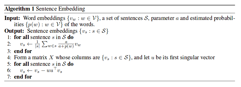
This is a striking illustration of how rigorously developed theoretical results can guide construction of simple algorithms in deep learning.
Final note: This series was based on the ICML 2018 tutorial on “Toward a Theory for Deep Learning” by Prof. Sanjeev Arora, which is why the discussion revolved mostly around the work done by his group. The papers themselves are not very trivial to understand, but the blog posts are more beginner friendly, and highly recommended. Several people criticize deep learning for being purely intuition-based, but I believe that will change soon, given that so much good research is being done to develop a theory for it.