Theory of Deep Learning: Role of Depth

In the previous posts of this series, we have looked at how stochastic gradient descent is able to find a good solution despite the nonconvex objective, and why overparametrized neural networks generalize so well. In this post, we will look at the titular property of deep networks, namely depth, and what role they play in the learning ability of the model.

An ideal result in this regard would be if we can show that there exists a class of natural learning problems (recall the idea of a “natural” problem from the first post) which cannot be solved with depth $d$ neural networks, but are solvable with at least one model of depth $d+1$. However, such a result is elusive at present, since we have already established that there exists no mathematical formulation of a “natural” learning problem.

However, there has been some advancement in establishing similar results in the case of less natural problems, and in this regard, the following papers are worth mentioning.

1. The Power of Depth for Feedforward Neural Networks by Eldan and Shamir
2. Benefit of Depth in Neural Networks by Telgarsky

I will now discuss both of these in some detail.

Role of depth for “less natural” problems

1. Approximating radial functions

At the outset, note that if we allow the neural network to be unbounded, i.e., have exponential width, even a 2-layer network can approximate any continuous function. As such, for our study, we only use “bounded” networks where the number of hidden layer units cannot be exponential in the dimension of input. With this understanding, we will look at the simplest case: we try to find a function (or a family of functions) that are expressible by a 3-layer network but cannot be expressed by any 2-layer network. Before we get into the details, we first look at what a 2-layer and 3-layer networks represent.

A 2-layer network represents the following function:

and a 3-layer network represents the following:

Here, $w$ is the size of the hidden layer and $\sigma$ is an activation function. The only constraint on $\sigma$ is that it should be “universal”, i.e., a 2-layer network should be able to approximate any Lipschitz function that is non-constant on a bounded domain for some $w$ (which need not be bounded). This constraint is satisfied by all the standard activation functions such as sigmoid and ReLU.

Under this assumption, the main result in the paper is as follows:

There exists a radial function $g$ depending only on the norm of the input, which is expressible by a 3-layer network of width polynomial in the input dimension, but not by any 2-layer neural network.

More importantly, apart from the universal assumption, this result does not depend on any characteristic of $\sigma$. Furthermore, there are no constraints on the size of the parameters $\mathbf{w}$. The only constraint worth noting is that $g$ must be a radial function.

To prove this result, we need to show 2 things:

1. $g$ can be approximated by a 3-layer neural network.
2. $g$ cannot be approximated by any 2-layer network of bounded width.

Part 1: This is trivial to show, since any radial function can be approximated by a 3-layer network. To do this, we compute the Euclidean norm $\lVert \mathbf{x} \rVert^2$ from the input $\mathbf{x}$ in the first layer using a linear combination of neurons. This is possible because the squared norm is just the sum of squares of all the components, and each squared component can be approximated in a finite range, for example, using the step function.

Once the norm is computed, the second layer can be used to approximate the required radial function using RBF nodes. This completes the construction.

Part 2: Let the input be taken from a probability distribution $\mu$, which has a density function $\phi^2(x)$, for some known function $\phi$. Suppose we are trying to approximate a function $f$ using a function $g$. Then, the distance between the functions can be given as

Now, we can replace $f\phi$ and $g\phi$ with their respective Fourier transforms since the Fourier transform is an isometric mapping (i.e., distance remains same before and after the mapping). Therefore, we get

While this replacement may seem arbitrary at first, it has a very clear motivation. We have done this because the Fourier transform of functions expressible by a 2-layer network has a very particular form, which we will use here. Specifically, consider the function

which is expressible by any 2-layer network. The component function $f_i (< \mathbf{v}_i,\mathbf{x} >)$ is constant in any direction perpendicular to $\mathbf{v}_i$ and so its Fourier transform is non-zero only in the direction of $\mathbf{v}_i$, and so the whole distribution is supported on $\bigcup_i \text{span}(\mathbf{v}_i)$. Now we just need to compute the support of $\hat{\phi}$, and then we can directly use the convolution-multiplication principle.

Since we haven’t yet chosen a density function, we choose $\phi$ to make the computation of support easier. Specifically, we choose $\phi$ to be the inverse Fourier transform of $\mathbb{1}\{x\in B\}$, which is the indicator function of a unit Euclidean ball. Then, $\hat{\phi}$ becomes $\mathbb{1}\{x\in B\}$ itself, and its support is simply the ball $B$. Using these, we get

which is basically the union of $k$ tubes passing through origin. This is because $\text{span}\{\mathbf{v}_i\}$ is just a straight line, and $B$ is a ball. Sum here means the direct sum, i.e., for every element $a \in A$ and $b \in B$, form a set of $a+b$. So we just put the Euclidean ball on every point on the line, which gives us a cylinder passing through the origin.

Since we are looking for a $g$ which cannot be approximated by the neural network, we try to make $\lVert f\phi - g\phi \rVert_{L_2}^2$ as large as possible. We have already seen what the support of $\hat{f\phi}$ looks like. Now, we want a $g$ such that

1. $g$ should have most of its mass away from the origin in all the directions, and
2. the Fourier transform $\hat{g}$ should be outside $B$.

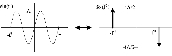
If $g$ is chosen as a radial function, the first criteria will be satisfied if we just put large mass away from the origin in one direction. To satisfy the second criteria, $g$ should have a high-frequency component. To see why, see the following figure which shows the sine curve and its Fourier transform.

The only thing that remains to be shown is that if $\hat{g}$ contains a significant mass away from the origin, then so does $\hat{g\phi}$. But this proof is somewhat technical in nature and I avoid it here for sake of simplicity.

This completes our proof for the result given in the paper. While this result is an important step in quantifying the role of depth in a neural network, it is still limited in that it only holds for radial functions. This is what I meant earlier by “less natural” problems, since in most of the common learning problems, the $(x,y)$ pairs are not generated from a simple radial distribution, and are much more complex in nature.

2. Exponential separation between shallow and deep nets

In the proof of the previous result, the key idea was to have a high-frequency component in the function required to be approximated. This means that the function was highly oscillatory. In this paper as well, a similar oscillation argument is used to prove another important result.

For every positive integer $k$, there exists neural networks with $\theta(k^3)$ layers, $\theta(1)$ nodes per layer, and $\theta(1)$ distinct parameters, which cannot be approximated by networks with $\mathcal{O}(k)$ layers and $o(2^k)$ nodes.

This result is proven using three steps.

1. Functions with few oscillations poorly approximate functions with many oscillations.
2. Functions computed by networks with few layers must have few oscillations.
3. Functions computed by networks with many layers can have many oscillations.

Approximation via oscillation counting

We will first look at a metric to count oscillations of a function. For this, consider the following graph which shows functions $f$ and $g$ which are defined from $\mathbb{R}$ to $[0,1]$.

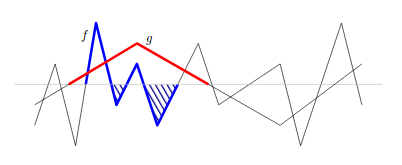
Here, the horizontal line denotes $y = \frac{1}{2}$. The classifiers $\tilde{f}$ and $\tilde{g}$ obtained from $f$ and $g$ perform binary classification according to the rule $\tilde{f}(x) = \mathbb{1}[f(x)\geq \frac{1}{2}]$. Let $\mathcal{I}_f$ denote the set of partitions of $\mathbb{R}$ into intervals so that the classifier $\tilde{f}$ is constant in each interval. Then, the crossing number is defined as

From our definition of $\tilde{f}$, this clearly means that $\text{Cr}(f)$ counts the number of times that $f$ crosses the line $y = \frac{1}{2}$, and hence the name. In this way, we formalize the notion of counting the number of oscillations of a function.

With this definition, if $\text{Cr}(f)$ is much larger than $\text{Cr}(g)$, then most piecewise constant regions of $\tilde{g}$ will exhibit many oscillations of $f$, and thus $g$ poorly approximates $f$.

Now we will prove the following lemma, where the counting number $\text{Cr}(f)$ is denoted by $s_f$ for sake of convenience.

\[\frac{\text{No. of regions of }\mathcal{I}_f \text{ where} ~ \tilde{f}\neq \tilde{g}}{s_f} \geq \frac{1}{2} - \frac{s_g}{s_f}\]

Now, if $s_f » s_g$, then the RHS approximately becomes $\frac{1}{2}$, which implies that for more than half of all the regions of $f$, $\tilde{g}$ classifies $x$ incorrectly, and so $g$ is a poor approximation of $f$.

Proof: We choose a region $J$ where $\tilde{g}$ is constant but $\tilde{f}$ alternates, such as the region where $g$ is red in the above figure. We denote by $X_J$ all the partitions of $\mathcal{I}_f$ that are contained in $J$. Since $f$ oscillates within $g$, this means that $\tilde{g}$ disagrees with $\tilde{f}$ for half of all $X_J$, i.e., at least $\frac{\vert X_J\vert-1}{2}$ in general.

In the LHS of the claim, we need to count all the regions of $\mathcal{I}_f$ where the classifiers disagree for all points in the region. From above, we have a lower bound on the number of such regions within one $J$. So now we just take sum over all $J \in \mathcal{I}_g$ to get

Now we need to bound $s_f$. For this, see that the total number of oscillations of $f$ are at least its number of oscillations within a single partition of $\mathcal{I}_g$ summed over all such partitions. I say “at least” because this will not include those partitions of $\mathcal{I}_f$ whose interior intersects with the boundary of an interval in $\mathcal{I}_g$. At most, there would be $s_g$ such partitions, and so

This means that $\sum_{J\in \mathcal{I}_g}\vert X_J\vert \geq s_f - s_g$. Using this bound in the previously obtained inequality, we get the desired result.

Few layers, few oscillations

Adding more nodes is similar to adding polynomials, while adding layers is like composition of polynomials. Adding polynomials yields a new polynomial with degree equal to the higher of the two and at most twice as many terms, but composing them (i.e. taking product) would yield a polynomial with higher degree and more than the product of terms. Clearly, composition would lead to more number of roots of the new polynomial. This suggests that adding layers should lead to a higher number of oscillations than adding nodes.

Let $f$ be a function computed by the neural network $\mathcal{N}((m_i,t_i,\alpha_i,\beta_i)_{i=1}^l)$, i.e. a network of $l$ layers where the $i$th layer has $m_i$ nodes, such that the activation function at each node is $(t,\alpha)-poly$ (a piecewise function containing $t$ parts where each piece is a polynomial of degree at most $\alpha$). Then, we claim that

Proof: We will prove this in two parts. First, we bound the counting number of a $(t,\alpha)-poly$ function, and then we will show that the function $f$ as computed by the above network is $(t,\alpha)-poly$.

For the first part, see that each piece of the function $f$ is a polynomial of degree at most $\alpha$, which means that each piece oscillates at most $1 + \alpha$ times. Since there are $t$ such pieces

Now it remains to show that the function $f$ computed by the network is indeed $(t,\alpha)-poly$. To see this, consider the function computed by a single layer. Each node in the layer computes a $(t,\alpha)-poly$ function, say $g_i$, and we apply a composition function, say $f$, on these $g_i$’s, which is a polynomial with degree at most $\gamma$. The final function computed by this layer is

To visualize such a composition, consider the following figure.

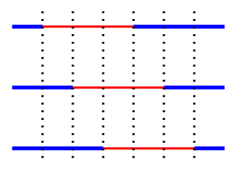
Here, each horizontal line denotes one node’s partition function, i.e., $\tilde{g_i}$. There are $k$ such lines with at most $t$ intervals each. The composition takes the union of all the partitions of all these lines. As such, the maximum number of intervals after composition will be equal to $kt$. Within each such interval, since we are taking a composition of a degree $\gamma$ polynomial with one with degree at most $\alpha$, the resulting polynomial has degree at most $\alpha \gamma$. Hence, $h$ is $(tk,\alpha\gamma)-poly$.

Since there are $l$ layers and the total number of nodes in the network is $m$, it implies there are $\frac{m}{l}$ nodes on average in each layer, and each node has at most $t$ intervals. So after every layer, the number of intervals gets multiplied by a factor of $\frac{mt}{l}$. Finally, the total number of intervals will be of the order $\left(\frac{mt}{l}\right)^l$.

Similarly, the degree of resulting function gets multiplied by $\alpha$ after every layer, so the final degree is of the order $\alpha^l$. Using the result shown in the first part, the resulting function will have a counting number bounded by $\mathcal{O}\left(\frac{tm\alpha}{l} \right)^l$.

The $\beta$ term comes due to technicalities associated with taking an activation function which is semi-algebraic rather than piecewise polynomial, but the proof technique remains the same.

Many layers, many oscillations

In the figure that I showed for explaining counting number, notice that oscillations usually (always?) mean repetitions of a triangle-like function (strictly increasing till some point and then strictly decreasing thereafter). Also, the usual functions computed by a single layer of most of the common neural networks are like these triangular functions.

In the last result, we used the composition of $(t,\alpha)-poly$ functions across several layers to bound the counting number of a network. Similarly in this section, we will use the concept of a $(t,[a,b])$-triangle. It represents a function which is continuous in $[a,b]$ and consists of $t$ triangle-like pieces. Also, since this function oscillates $2t$ times, its counting number is $2t+1$.

Now it remains to show that the composition of 2 such functions gives a similar function (which is a similar technique to what we used earlier). More formally, we will prove this claim.

Claim: If $f$ is a $(s,[0,1])$-triangle and $g$ is a $(t,[0,1])$-triangle, then $f \circ g$ is a $(2st,[0,1])$-triangle.

Proof: First, we note that $f \circ g$ is continuous in $[0,1]$ since a composition of continuous functions is continuous in the same domain.

Now, consider any odd (i.e., strictly increasing) interval $g_j$ of $g$. Suppose $(a_1,\ldots,a_{2s+1})$ are the interval boundaries of $f$. Since the range of $g_j$ is $[0,1]$, $g_j^{-1}(a_i)$ exists for all $i$ and is unique, since $g_j$ is strictly increasing. Let $a_i^{\prime}=g_j^{-1}(a_i)$, i.e., $g_j(a_i^{\prime})=a_i$. If $i$ is odd, the composition $f \circ g_j(a_i^{\prime}) = f(a_i)=0$, and $f \circ g_j$ is strictly increasing in $[a_i^{\prime},a_{i+1}^{\prime}]$, since $g_j$ is strictly increasing everywhere and $f$ is strictly increasing in $[a_i,a_{i+1}]$. By a similar argument, if $i$ is even, $f \circ g_j$ is strictly decreasing along $[a_i^{\prime},a_{i+1}^{\prime}]$. In this way, we get $2s$ triangular pieces for a single $g_j$, and so the overall composition $f \circ g$ has $2st$ triangular pieces.

Having shown this, it is easy to see that if there are $l$ layers and each layer computes a $(t,[0,1])$-triangle, the final layer will output a $((2t)^l,[0,1])$-triangle. In this way, the counting number of the overall function becomes $(2t)^l + 1$.

Implicit acceleration by overparametrization

In the previous section, we have seen some results which show that depth plays a role in the expressive capacity of neural networks. Specifically, we saw that:

1. Radial functions can be approximated by depth-3 networks but not with depth-2 networks.
2. Functions expressible by $\theta(k^3)$-depth networks of constant width cannot be approximated by $\mathcal{O}(k)$-depth networks with polynomial width.

In this section, we will look at a new paper from Arora, Cohen, and Hazan that suggests that, sometimes, increasing depth can speed up optimization (which is rather counterintuitive given the consensus on expressiveness vs. optimization trade-off), i.e., depth plays some role in convergence. Furthermore, this acceleration is more than what could be obtained by commonly used techniques, and is theoretically shown to be a combination of momentum and adaptive regularization (which we will discuss later).

To isloate convergence from expressiveness, the authors focus solely on linear neural networks, where increasing depth has no impact on the expressiveness of the network. This is because in such networks, adding layers manifests itself only in the replacement of a matrix parameter by a product of matrices – an overparameterization.

Equivalence to adaptive learning rate and momentum

The first result that we prove is the following.

Overparametrized gradient descent with small learning rate and near-zero initialization is equivalent to GD with adaptive learning rate and momentum terms.

Proof: This can be seen by simple analysis of gradients for an $l_p$-regression with parameter $\mathbf{w}\in \mathbb{R}^d$. The loss function can be given as

Now, if we add a scalar parameter, the new parameters are $\mathbf{w}_1$ and $w_2 \in \mathbb{R}$, i.e., $\mathbf{w} = w_2 \mathbf{w}_1$, and we can write the new loss function as

We can now compute the gradients of the objective with respect to the parameters as

The update rules for $\mathbf{w}_1$ and $w_2$ can be given as

and the updated parameter $\mathbf{w}$ is

We can ignore $\mathcal{O}(\eta^2)$ since the learning rate is assumed to be low. Also, we take $\rho^{(t)} = \eta(w_2^{(t)})^2$ and $\gamma^{(t)}=\eta(w_2^{(t)})^{-1}\nabla_{w_2^{(t)}}$, so the update becomes

Since $\mathbf{w}$ is initialized near $0$, it is essentially a weighted combination of the past gradients at any given time, i.e., $\gamma^{(t)}\mathbf{w}^{(t)} = \sum_{\tau=1}^{t-1}\mu^{(t,\tau)}\nabla_{\mathbf{w}^{(\tau)}}$.

This is similar to the momentum term in the popular momentum algorithm for optimization (see this earlier post for an overview), and the learning rate term $\rho^{(t)}$ is time-varying and adaptive.

Update rule for end-to-end matrix

The next derivation is a little more involved, and I defer the reader to the actual paper for the detailed proof. I will give a brief outline here.

Suppose we have a depth-$N$ linear network such that the weight matrices are given by $W_1,\ldots,W_N$. Let $W_e$ denote the final end-to-end update matrix. The authors use differential techniques to compute an update rule for $W_e$. For this, the important assumption is that $\eta^2 \approx 0$. When step sizes are taken to be small, trajectories of discrete optimization algorithms converge to smooth curves modeled by continuous-time differential equations.

After obtaining such a differential equation, integration over the $N$ layers gives the derivative of $W_e$, which is then transformed back to the discrete update rule given as

Let us break down this expression. The first part is similar to a weight-decay term for a 1-layer update. The second part also has the derivative w.r.t parameters, but it is multiplied by some preconditioning terms. On further inspection of these terms, it is found that their eigenvalues and eigenvectors depend on the singular value decomposition of $W_e$. Qualitatively, this means that these multipliers favor the gradient along those directions that correspond to singular values whose presence in $W_e$ is stronger. If we assume, as is usually the case in deep learning, that the initialization was near 0, this means that these multipliers act similar to acceleration and push the gradient along the direction already taken by the optimization.

For further reading, check out the author’s blog post about the paper.

To summarize, we looked at three recent papers which prove results on the role of depth in expressibility and optimization of neural networks. People often think that working on the mathematics of deep learning would require complex group theory formalisms and difficult techniques in high-dimensional probability, but as we saw in the proofs of some of these results (especially in Telgarsky’s paper), a lot can be achieved using simple counting logic and concentration inequalities.