Theory of Deep Learning: Optimization

I only just got around to watching the ICML 2018 tutorial on “Toward a Theory for Deep Learning” by Prof. Sanjeev Arora. In this and the next few posts, I will discuss the subject in some detail, including the referenced papers and blogs. Very conveniently, the talk itself was divided into 5 parts, and I will structure this series accordingly.

At the outset, we should understand that a number of important concepts in deep learning are already shaped by optimization theory. Backpropagation, for instance, is basically just a linear time dynamic programming algorithm to compute gradient. Recent methods for gradient descent, such as momentum, Adagrad, etc. (see this post for a quick overview) are obtained from convex optimization techniques. However, over the last decade, the deep learning community has come up with several models based on intuition mostly, that do not have any theoretical support yet.

The goal, then, is to find theorems that support these intuitions, leading to new insights and concepts.

In this first part of the series, we will try to understand why (and how) deep learning almost always finds decent solutions to problems that are highly nonconvex.

Possible goals for optimization

Any neural network essentially tries to minimize a loss function. However, in almost all cases, this loss function is highly nonconvex (and sometimes NP-hard), which means that no provably polytime algorithm exists for its optimization. Even so, deep networks are quite adept at finding an approximately good solution.

Whenever the gradient $\nabla$ is non-zero, there exists a descent direction. As such, a possible goal for the network may be any of the following (in increasing order of difficulty):

1. Finding a critical point, i.e. $\nabla = 0$.
2. Finding a local optimum, i.e. $\nabla = 0$ and $\nabla^2$ is positive semi-definite.
3. Finding a global optimum.

Furthermore, this descent may be from several possible initializations, namely all points, random points, or specially-chosen points. Now, if there are $d$ parameters (weights) to be optimized, we say that the problem is in $\mathbb{R}^d$ space. It is usually visualized by the following sea-urchin figure (or a $d$-urchin figure, according to Prof. Arora).

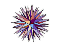
In $\mathbb{R}^d$ space, there exit exp($d$) directions which can be explored to find the optimal solution, which makes the naive approach infeasible. Also, we cannot use non black box approaches to prune the number of explorations, since there is no clean mathematical formulation for the problem.

But what does this mean? This means that problems in deep learning are usually of the kind where, given pixels of an image, you have to label it as a cat or a dog. Such an $(x_i,y_i)$ has no mathematical meaning. This means that we do not understand the inherent landscape of the problem we are trying to solve, and so no special pruning can be done.

This, combined with the nonconvex nature of the loss function, also means that it becomes infeasible to find a global optimum for the optimization problem. As such, we have to settle for goals 1 and 2, i.e. a critical point or a local optimum.

Finding critical points

The update function for a parameter $\theta$ is given as

If the second derivative $\nabla^2$ is high, $\nabla f(\theta_t)$ will vary a lot, and we may miss the actual critical point. To prevent this, it is advisable to take small steps.

But how do we quantify small? In other words, how do we determine a good learning rate for the optimization problem? For this, we again look at $\nabla^2$, which will determine the smoothness of the function. Suppose there exists a $\beta$ such that the Hessian $-\beta I \leq \nabla^2 f(\theta) \leq \beta I$, where $I$ is the identity matrix. Essentially, a higher $\beta$ means that $\nabla^2$ varies more, and so the learning rate should be lower. From this understanding, we can prove the following claim.

Claim (Nesterov 1998): If we choose $\eta = \frac{1}{2\beta}$, we can achieve $

\nabla f

<\epsilon$ in number of steps proportional to $\frac{\beta}{\epsilon^2}$.

Proof: See the proof of Lemma 2.8 here (see Definition 2.7). So a single update reduces the function value by at least $\frac{\epsilon^2}{2\beta}$. Therefore, it would take $\mathcal{O}(\frac{\beta}{\epsilon^2})$ steps to arrive at a critical point.

Evading saddle points

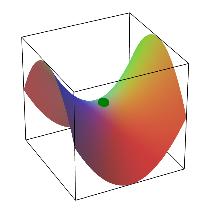
While we have a theoretical upper limit for the time taken for convergence at a critical point, this is still problematic since it may be a saddle point, i.e., the function value is minimum in $d-1$ directions but maximum in one direction. Such a surface literally looks like a saddle as follows.

An important question, then, is how to evade saddle points while looking for critical points. This question is explored in a series of papers and corresponding blog posts on Prof. Arora’s blog.

1. Polynomial time guarantee for GD to escape saddle points (based on this paper)
2. Random initialization for asymptotically avoiding saddle points (based on this paper)
3. Perturbing gradient descent (based on this paper)

Here I will try to summarize these discussions in several bullet points.

• Most learning problems have exponentially many saddle points. Learning problems usually involve searching for $k$ components, for example clustering, $k$-node hidden layer in a neural network, etc. Suppose $(x_1,x_2,\ldots,x_k)$ is an optimal solution. Then, $(x_2,x_1,\ldots,x_k)$ is also an optimal solution, but the mean of these is not an optimal solution. This suffices to show that the learning problem is nonconvex, since for a convex function, the average of optimal solutions is also optimal. Furthermore, we can keep swapping the $k$ components to obtain exponential optimal solutions. Saddle points lie on the paths joining these isolated solutions, and hence, are exponential in number themselves.

• Hessians can be used to evade saddle points. Consider the second order Taylor expansion given below. If there exists a direction where $\frac{1}{2}(y-x)^T \nabla^2 f(x)(y-x)$ is significantly less than 0, then using this update rule can avoid saddle points. Such saddle points are called “strict,” and for these, methods such as trust region algorithms and cubic regularization can find the local optimum.

• Noisy gradient descent converges to local optimum in polynomial number of steps. Although the Hessian method provides a theoretical way to escape saddle points, the computation of $\nabla^2$ is still expensive. Suppose we put a ball on a saddle point. Then, giving it only a slight push will move it away from the saddle. This intuition leads to the notion of “noisy” GD, i.e., $y = x - \eta \nabla f(x) + \epsilon$, where $\epsilon$ is a zero-mean error, which is often cheaper to compute than the true gradient. The authors in also prove the theorem in the paper, but it is very non-trivial.

• It is hard to converge to a saddle point. Furthermore, a random initialization of GD will asymptotically converge to a local minimum, rather than other stationary points. In (2), Ben Recht emphasized that “even simple algorithms like gradient descent with constant step sizes can’t converge to saddle points unless you try really hard.” To prove this, they use the Stable Manifold Theorem, taking $x^{\ast}$ to be an arbitrary saddle point and showing that this measure was always zero.

The Stable Manifold theorem is concerned with fixed point operations of the form $x^{(k+1)}=\psi(x^{(k)})$. It quantifies that the set of points that locally converge to a fixed point $x^{\ast}$ of such an iteration have measure zero whenever the Jacobian of $\psi$ at $x^{\ast}$ has eigenvalues bigger than 1.

In fact, it has been shown long back that additive Gaussian noise is sufficient to prevent convergence to saddles, without even assuming the “strictness” criteria of (1).

Now that it is clear that GD can avoid saddle points almost certainly, it remains to be seen whether it is efficient in doing so. The paper (1), although it did show a poly-time convergence for the noisy GD, was still inefficient because its polynomial dependency on the dimension $n$ and the smallest eigenvalue of the Hessian are impractical. The paper (3) further improves this aspect of the problem.

• A perturbed form of GD, under an additional Hessian-Lipschitz condition, converges to a second-order stationary point in almost the same time required for GD to converge to a first-order stationary point. Furthermore, the dimensional dependence is only polynomial in $\log(d)$.

• Finally, recent work definitely shows that PGD is much better than GD with random initialization, since the latter can be slowed down by saddle points, taking exponential time to escape. This is because if there are a sequence of closely-spaced saddle points, GD gets closer to the later ones, and takes $e^i$ iterations to escape the $i^{th}$ saddle point. PGD, on the other hand, escapes each saddle point in a small number of steps regardless of history.

Summary: Although most learning problems have exponentially many saddle points, they are hard to converge to, and even random initializations can escape them. They take a long time for this escape though, which is why using perturbations is more efficient, and actually as efficient as GD for first-order stationary points. Therefore, using information from Hessians is not necessary to escape saddle points efficiently.

Second-order methods for local optimum

Although we have established that Hessians are unnecessary for finding the local optimum, it would still be enlightening to look at some approaches for the same.

Agarwal et. al ‘17 proposed LiSSA, or Linear (time) Stochastic Second-order Algorithm. The basic update rule is

i.e. the gradient is scaled by the inverse of the Hessian, which intuitively makes sense as discussed earlier. Although backpropagation can compute the Hessian itself in linear time, we require the inverse. In this paper, the LiSSA algorithm uses the idea that $(\nabla^2)^{-1} = \sum_{i=1}^{\infty}(I - \nabla^2)^i$, but with finite truncation.

Carmon et al. ‘17 further improved upon the $\mathcal{O}(\frac{1}{\epsilon^2})$ guarantee provided by gradient descent for $\epsilon$-first-order convergence, without any need for Hessian computation. They use two competing techniques for this purpose. The first has already been discussed above:

If the problem is locally non-convex, the Hessian must have a negative eigenvalue. In this case, under the assumption that the Hessian is Lipschitz continuous, moving in the direction of the corresponding eigenvector must make progress on the objective.

The second technique is more novel. They show that if the Hessian’s smallest eigenvalue is at least $-\gamma$, we can apply proximal point techniques and accelerated gradient descent to a carefully constructed regularized problem to obtain a faster running time.

While their approach is asymptotically faster than first-order methods, it is still empirically slower. Furthermore, it doesn’t seem to find better quality neural networks in practice.

Understanding the landscape: Matrix completion

Very early on in this post, we established that in deep learning problems, the landscape is unknown, i.e. the problem does not have a meaningful mathematical formulation. In this vein, we now look at a paper that develops a new framework to capture the landscape. In particular, we will approach this problem in the context of matrix completion. (Interestingly, this paper is again from Rong Ge, who first showed polytime convergence to local minimum for noisy GD.)

But first, what is matrix completion. Matrix completion is a learning problem wherein the objective is to recover a low-rank matrix from partially observed entries. The mathematical formulation of the problem is:

where $E$ is the set of observed entries. Most approaches to solve this problem represent it in the form of the following nonconvex objective.

Here, $R(X)$ is a regularization term which ensures that no single row of $X$ becomes too large, otherwise most observed entries will be 0.

Ge showed in an earlier paper that in case of matrix completion (others have shown the same result for other problems like tensor decomposition and dictionary learning), all local minima are also global minima.

For matrix completion, all local minima are also global minima.

In the present paper, the authors proposed the new insight that for the case of the matrix completion objective as defined above, the function $f$ is quadratic in $X$, which means that its Hessian w.r.t $X$ is constant. Furthermore, any saddle point has at least one strictly negative eigenvalue in its Hessian. Together, these ensure that simple local search algorithms can find the desired low rank matrix from an arbitrary starting point in polynomial time with high probability.

These advances, while mathematically involved, show that characterizing the various stationary points of the learning objective can be helpful in providing theoretical guarantees for learning algorithms. While I have avoided proof details for the several important theorems here, I will try to understand and explain them lucidly in some later post.