Theory of Deep Learning: Generalization

In Part 1 of this series, based on the ICML 2018 tutorial on “Toward a Theory for Deep Learning” by Prof. Sanjeev Arora, we looked at several aspects of optimization of the nonconvex objective function that is a part of most deep learning models. In this article, we will turn our attention to another important aspect, namely generalization.

A distinguishing feature of most modern deep learning architectures is that they generalize to test cases exceptionally well, even though the number of parameters is far greater than the number of training samples. VGG19, for instance, which has approximately 20 million weights to be tuned, gives $\sim 93\%$ classification accuracy on CIFAR-10, which has only 50000 training images. If you have studied statistical learning theory (see my previous blogs on the topic), this behavior is extremely counter-intuitive, and begs the question: why don’t deep neural networks overfit even with small number of training samples?

Before we try to understand the reason, let us look at a popular folklore experiment that is described in Livni et al ‘14 related to over-specification.

For sufficiently over-specified networks, global optima are ubiquitous and in general computationally easy to find.

To see this, we fix a depth-2 neural network (i.e. a network with 1 hidden layer) consisting of $n$ hidden nodes. We provide random inputs to the network and obtain their corresponding output. Now, take a randomly initialized neural network with the same architecture as the above, and train it using the input-output pairs obtained earlier. It is found that this is really difficult to achieve. However, if we take a large number of hidden nodes, the training becomes easier.

Although this result has been known and verified empirically for some time, it remains to be proven theoretically. This is a striking example of the difficulty of proving generalization guarantees in deep learning.

Effective capacity of learning

The capacity of a learning model, in an abstract sense, means the complexity of training samples that it can fit. For instance, a quadratic regression has inherently more capacity than linear regression, but is also more prone to overfitting. Furthermore, the effective capacity can be thought of as analogous to the number of bits required to represent all possible states that the hypothesis class contains. For this reason, the capacity is approximately the log of the number of apriori functions in the hypothesis class.

We will now see a general result that is true for learning models including deep neural networks.

Claim: Test loss - training loss $\leq \sqrt{\frac{N}{m}}$, where $N$ is the effective capacity and $m$ is the number of training samples.

Proof: First let us fix our neural network $\theta$ and its parameters. Suppose we take an i.i.d sample $S$ containing $m$ data points. Consider Hoeffding’s inequality: If $x_1,\ldots,x_m$ are $m$ i.i.d samples of a random variable $X$ distributed by $P$, and $a\leq x_i \leq b$ for every $i$, then for a small postive non-zero value $\epsilon$:

\[P\left( \mathbb{E}_{X \sim P} - \frac{1}{m}\sum_{i=1}^m x_i \right) \leq 2\exp \left( \frac{-2m\epsilon^2}{(b-a)^2} \right)\]

We can apply this inequality to our generalization probability, assuming that our errors are bounded between 0 and 1 (which is a reasonable assumption, as we can get that using a 0/1 loss function or by squashing any other loss between 0 and 1) and get for a single hypothesis $h$:

\[P(|R(h) - \hat{R}(h)| > \epsilon) \leq 2\exp (-2m\epsilon^2),\]

where $R(h)$ denotes generalization error and $\hat{R}(h)$ denotes empirical error on the sample.

However, this is not the true generalization bound. This is because we have first fixed out network and we are then choosing the sample i.i.d. However, in a real learning problem, we are given the sample $S$ and we have to learn the parameters to best fit this sample. Therefore, to obtain the actual generalization bound, we take the union bound over all possible neural net configurations $\mathcal{W}$. Now, equating the RHS with the confidence $\delta$, we get

\[\begin{align} & 2\mathcal{W}\exp(-2m\epsilon^2) \leq \delta \\ \Rightarrow & -2m\epsilon^2 \leq \log \frac{\delta}{2\mathcal{W}} \\ \Rightarrow & \epsilon \geq \sqrt{\frac{\log \frac{2\mathcal{W}}{\delta}}{2m}}, \end{align}\]

which completes the proof.

In statistical learning theory, the most popular metrics for measuring the capacity of a model are Rademacher complexity and VC dimension, which I have explained in this post. I will quickly summarize them here.

Rademacher complexity: It is a measure of how well the model can fit a random assignment of labels. Its mathematical formulation is:

Essentially, it denotes an expectation of the best possible average correlation that the random labels have with any function present in the hypothesis class $G$. Therefore, a higher Rademacher complexity would imply that the function class $G$ is able to fit a random assignment of labels well, and vice versa. This is because the more complex a class $G$ is, higher is the probability that it would have some $g$ which correlates well with random noise.

The generalization error $R(h)$ can be written in terms of R.C. as

where $\hat{R}(h)$ is the empirical error, $\delta$ is the confidence, and $m$ is the number of training samples.

VC dimension: It is the size of the largest set that can be fully shattered by $G$. By shattering, we mean that $G$ can classify the given set in all possible ways. As such, higher the VC-dimension, more is the capacity of the hypothesis class. We can bound the generalization error in terms of the VC-dimension of the hypothesis class as

Although these metrics are well established in learning theory, they fail for deep neural networks since they are usually equally vacuous, i.e, the upper bound is greater than 1. This means that the bounds are so large that they are meaningless, since error can never exceed 1, and in practice the generalization error of the networks is many orders of magnitude less than these bounds.

Deep networks have “excess capacity”

As mentioned earlier, deep neural networks generalize surprisingly well despite having a huge number of parameters. They can be shown by the dotted red line (figure taken from tutorial slides) in the following popular figure which is often found in textbooks.

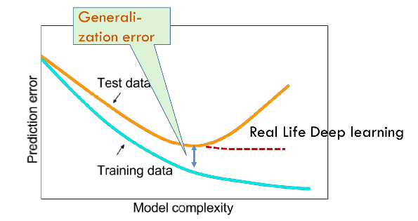
Other learning models with a “high capacity” would follow the general trend and fail to generalize well, which may be evidence that somehow, the large number of parameters in deep networks is not necessarily translating to a high capacity. For a long time, it was believed that a combination of stochastic gradient descent and regularization eliminates the “excess capacity” of the neural network.

But this belief is wrong!

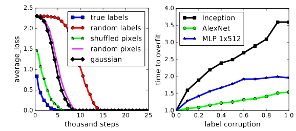
In their ICLR ‘17 paper (which I have previously discussed in this post), Zhang et. al., in a series of well-designed experiments, showed that deep networks do retain this excess capacity. From Prof. Arora’s blog post on the subject: “Their main experimental finding is that if you take a classic convnet architecture, say Alexnet, and train it on images with random labels, then you can still achieve very high accuracy on the training data. (Furthermore, usual regularization strategies, which are believed to promote better generalization, do not help much.) Needless to say, the trained net is subsequently unable to predict the (random) labels of still-unseen images, which means it doesn’t generalize.”

An interesting (and provable) guarantee that the paper contains is the following theorem: There exists a two-layer neural network with ReLU activations and $2n+d$ weights that can represent any function on a sample of size $n$ in $d$ dimensions.

In a related paper published recently, it was shown that the “excess capacity” is not just limited to deep networks, since even linear models possess this feature. Furthermore, when it comes to fitting noise, there are some interesting similarities between Laplacian kernel machines and ReLU networks. But before we get to that, I will briefly define Laplacian and Gaussian kernels. (For an overview of several kernel functions, check out this article.)

Kernel Methods

Kernel methods map the data into higher-dimensional spaces, in the hope that in this higher-dimensional space the data could become more easily separated or better structured. However, when we talk about transforming data to a higher dimension, called a $z$-space, an actual transformation would involve paying computation costs. To avoid this, we need to look at what we actually want from the $z$-space.

Support Vector Machines (SVMs), which are among the most popular kernel-based methods for classification, involve solving for the following Lagrangian.

\[\mathcal{L}(\alpha) = \sum_{n=1}^N \alpha_n - \frac{1}{2}\sum_{n=1}^N \sum_{m=1}^M y_n y_m \alpha_n \alpha_m z_n^T z_m\]

under the constraints $\alpha_n \geq 0 \forall n$ and $\sum_{n=1}^N \alpha_n y_n = 0$. On solving this, we get the boundary as

\[g(x) = \text{sgn}(w^T z + b)\]

where $w = \sum_{z_n \in SV} \alpha_n y_n z_n$.

We can see from this that the only value we need from the $z$-space is the inner product $z^T z^{\prime}$. If we can show that obtaining this inner product is possible without actually going to the $z$-space, we are done.

It turns out that this is indeed possible, and there are several such functions, known as kernel functions, which can be written as the inner product in some space. The only constraint on the $z$-space is that it should exist. Interestingly, kernels such as the radial basis function (RBF) kernel exist in an $\infty$-dimensional space. Furthermore, in order for the problem to be convex and have a unique solution, it is important to select a positive semi-definite kernel, i.e., whose kernel matrix contain only non-negative eigenvalues. Such a kernel is said to obey Mercer’s theorem.

Now that we have some idea what kernels are, let us look at Laplacian and Gaussian kernels.

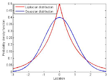
• Laplacian kernel: It is mathematically defined as

• Gaussian kernel: Its mathematical formulation is

Both the Laplacian and Gaussian kernels are examples of the radial basis function kernels. The difference lies only in the parameter $\sigma$. Since the Gaussian depends on the square of this parameter, it is more sensitive to changes in $\sigma$ than the Laplacian.

The authors found in their empirical evaluations that Laplacian kernels were much more adept at fitting random labels than Gaussian kernels. This property may be attributed to the inherent non-smoothness of Laplacians as opposed to the Gaussians being smooth. This discontinuity in derivative is reminiscent of that for ReLU units, which, as we saw above, were found to fit random labels exceptionally well. As such, the conjecture is that the radial structure of the kernels, as opposed to the specifics of optimization, plays a key role in ensuring strong classification performance.

Another take-away from this paper is that they establish stronger bounds for classification performance of kernel methods. If understanding kernels can indeed lead to a better understanding of deep learning, then maybe these bounds will lead to tighter bounds for the effective capactity of deep neural networks.

Other notions of generalizability

We now look at 2 other concepts that seek to explain why deep neural networks generalize well: flat minima, and noise stability.

Flat minima

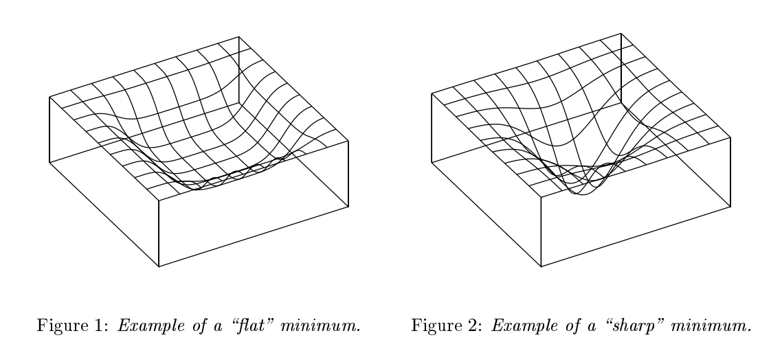
Hochreiter and Schmidhuber first conjectured that the flatness of the local minima found by the stochastic gradient descent may be an indicator of its generalization performance. Sharpness of a minimizer can be characterized by the magnitude of the eigenvalues of $\nabla^2 f(x)$, but since the computation of this quantity is expensive, Keskar et. al. defined a new metric for sharpness that is easier to compute.

Given $x \in \mathbb{R}^n$, $\epsilon > 0$, and $A \in \mathbb{R}^{n \times p}$, the $(C_{\epsilon},A)$-sharpness of $f$ at $x$ is defined as

The metric is based on exploring a small neighborhood of a solution and computing the largest value that $f$ can attain in that neighborhood. We use that value to measure the sensitivity of the training function at the given local minimizer.

Intuitively, flat minima have lower description lengths (since less information is required to represent a flat surface), and consequently, fewer number of models are possible with this length. The effective capactiy thus becomes less, and so the hypothesis is able to generalize well.

However, recent research suggests that flatness is sensitive to reparametrizations of the neural network: we can reparametrize a neural network without changing its outputs while making sharp minima look arbitrarily flat and vice versa. As a consequence the flatness alone cannot explain or predict good generalization.

As Prof. Arora pointed out in his talk, most of the existing theory that tries to explain generalization is only doing a “postmortem analysis”. This means that they look at some property $\phi$ that is seemingly possessed by a few neural networks that generalize well, and they argue that the generalization is due to this property. The notion of “flat minima” is a prime example of this. However, correlation is not causation. Instead of such a qualitative check, the theoretical approach would be to use the property $\phi$ to compute an upper bound on the number of possible neural networks that would generalize well with this property. This computation is very nontrivial and is therefore ignored.

Noise stability

While flat minima was an old concept, the notion of noise stability is a very recent formalization for the same, proposed in Prof. Arora’s ICML’18 paper. Essentially, it means that if we add some zero-mean Gaussian noise at an intermediate output of a neural network, the noise gets attenuated as the signal moves to higher layers. Therefore, the capacity of a network to fit random noise can be measured by adding a Gaussian noise at an intermediate layer and measuring the change in output at higher layers.

This is also biologically inspired, since neurologists believe that single neurons are extremely susceptible to errors. However, the fact that we still function well suggests that there must be some mechanism to attenuate these errors.

Noise stability implies compressibility.

First, what is meant by compression of a neural network? Given a network $C$ with $N$ parameters and some training loss, compression means obtaining a new network $C^{\prime}$ containing $N^{\prime}$ parameters ($N^{\prime} < N$), such that the training loss effectively remains the same. From the generalization claim proved earlier, this compression would mean better generalization capability for the network $C^{\prime}$.

Now, let us consider a depth-2 network consisting only of linear transformations. This network can be represented by some matrix $M$, which transforms input $x$ to output $Mx$.

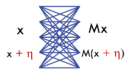
In the above figure, $\eta$ is a zero-mean Gaussian noise that is added to the input. We say that the matrix $M$ is noise stable, i.e. $M(x+\eta)\approx Mx$. This means that $\frac{\vert Mx\vert}{\vert x\vert} » \frac{\vert M\eta\vert}{\vert\eta\vert}$. Here, the value $\frac{\vert Mx\vert}{\vert x\vert}$ is at most equal to the largest singular value of $M$, which we denote by $\sigma_{\max}(M)$. The RHS is approximately $\frac{(\sum_i (\sigma_i (M))^2)^{\frac{1}{2}}}{\sqrt{n}}$ where $\sigma_i(M)$ is the $i$th singular value of $M$ and $n$ is dimension of $Mx$. The reason is that gaussian noise divides itself evenly across all directions, with variance in each direction $1/n$. Thus,

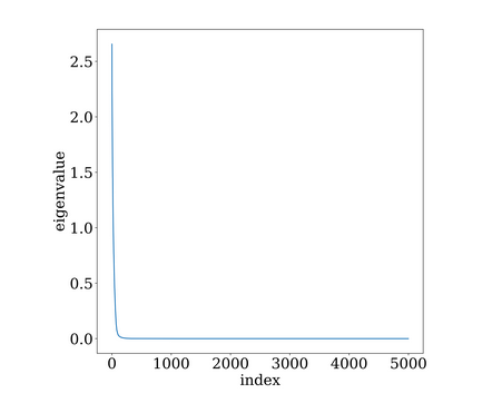
The ratio of the LHS to the RHS in the above inequality is known as the stable rank. Higher the stable rank, more uneven is the distribution of singular values in the matrix. This is easily seen since the highest singular value is much larger than the RMS of all the singular values, something similar to the following figure.

The actual signal $x$ is usually correlated with the eigenvectors corresponding to the larger singular values, and as such, the other directions can be ignored without any loss in performance. This is similar to feature selection by a principal component analysis approach.

Nonvacuous bounds for true capacity

We have earlier seen that most of the classical metrics used for bounding the generalization error in learning systems prove to be vacuous in case of deep neural networks. The following blog posts by Prof. Arora discuss this issue in some detail and also introduce a new generalization bound based on the compressibility of neural networks explained in the previous section.

1. Generalization theory and deep nets, an introduction
2. Proving generalization of deep nets via compression

In this section, I will discuss two approaches for computing nonvacuous bounds for deep networks. The first is from Dziugaite and Roy, and the second is from Prof. Arora’s ICML’18 paper mentioned previously.

As discussed earlier, a common framework for addressing this problem would involve showing under certain assumptions that either SGD performs implicit regularization, or that it finds a solution with some known structure connected to regularization. Once this is found, a nonvacuous bound for the generalization error of such models would have to be determined.

1. PAC-Bayes approach

The first question is how to identify structure in the solutions found by SGD? For this, we again turn to the old notion of flat minima. If SGD finds a flat minima, it means that the solution is surrounded by a large volume of solutions that are nearly as good. If we then represent these nearby solutions by some distribution and pick an average classifier from this distribution, it would be very likely that its generalization error is very close to that of the true solution.

This concept is very similar to the PAC-Bayes theorem, which informally bounds the expected error of a classifier chosen from a distribution $Q$ in terms of its KL divergence from a priori fixed distribution $P$. But first, what is KL divergence?

Kullback-Leibler divergence

It is a metric that compares the similarity between two probability distributions. Mathematically, it is the expectation of the log difference between the probability of data in the original distribution $p$ and the approximating distribution $q$.

\[\begin{align} KL(p||q) &= \mathbb{E}(\log p(x) - \log q(x)) \\ &= \sum_{i=1}^N p(x_i)(\log p(x_i) - \log q(x_i)) \end{align}\]

In information theory, the most important notion is that of entropy, which represents the minimum number of bits required to encode some information, and is mathematically represented as

\[H = -\sum_{i=1}^N p(x_i)\log p(x_i).\]

As such, the KL divergence can be seen to compute how many bits of information will be lost in approximating a distribution $p$ with another distribution $q$.

The PAC-Bayes bound is given as

where $\hat{e}(Q,S_m)$ is the empirical loss of $Q$ w.r.t some i.i.d sample $S_m$, and $e(Q)$ is the expected loss. If we now find a $Q$ that minimizes this value, we are likely to find a minima that generalizes well and has a nonvacuous bound. This is exactly what is proposed in the paper.

On a binary variant of MNIST, the computed PAC-Bayes bounds on the test error are in the range 16-22%. While this is a loose bound (actual bounds are around 3%), it is still surprising to find a non-trivial numerical bound for a model with such a large capacity on so few training examples. The authors comment that these are, in all likelihood, “the first explicit and nonvacuous numerical bounds computed for trained neural networks in the deep learning regime”.

2. Compressibility approach

Although the PAC-Bayes bound is nonvacuous, it is still looser than actual sample complexity bounds computed empirically. Instead, Arora et al. introduce a new compression framework to address this problem. Earlier while discussing noise stability, we have already seen that if we can compress a classifier $f$ without decreasing the empirical loss, it becomes much more generalizable according to the fundamental theorem proved earlier.

We say that $f$ is $(\gamma,S)$-compressible using helper string $s$ if there exists some other classifier $g_{A,s}$ on a class of parameters $A$ such that the classification loss of $f$ on every $x \in S$ differs from that of $g_{A,s}$ by at most $\gamma$. Here, $s$ is fixed before looking at the training sample, and is often just for randomization.

Then, the main theorem in the paper is as follows: If $f$ is $(\gamma,S)$-compressible using helper string $s$, then with high probability,

where $A$ is a set of $q$ parameters each having at most $r$ discrete values, $L_0 (g_A)$ is the generalization loss of compressed classifier, and $\hat{L}_{\gamma}(f)$ is the empirical estimate of the marginal loss of original classifier. Note that the bound is for the compressed classifier, but the same is also true for earlier works (like the PAC-Bayes approach). The proof is very elementary and uses just simple concentration inequalities.

Proof: First, using Hoeffding’s inequality, we can write

\[P(L_0 (g_A) - \hat{L}_0 (g_A) \geq \epsilon) \leq 2\exp(-2m\epsilon^2).\]

Taking $\epsilon = \sqrt{\frac{q \log r}{m}}$, we get, with probability at least $1 - \exp(-2q\log r)$,

\[L_0 (g_A) \leq \hat{L}_0 (g_A) + \mathcal{O}\left( \sqrt{\frac{q \log r}{m}} \right).\]

Next, by definition of $(\gamma,S)$-compressibility, we can write

\[\lvert f(x)[y] - g_A(x)[y] \rvert \leq \gamma.\]

This means that as long as the original function has margin at least $\gamma$, the new function classifies the example correctly. Therefore,

\[\hat{L}_0 (g_A) \leq \hat{L}_{\gamma}(f).\]

Combining this with the earlier inequality, we immediately get the result.

In addition to providing a tighter generalization bound for fully connected networks, the paper also proposes some theory for convolutional nets, which have been notoroiusly difficult to theorize. For details, readers are suggested to refer to the paper.