Theory of Deep Learning: Generative Models

Till now, in this series based on the ICML 2018 tutorial on “Toward a Theory for Deep Learning” by Prof. Sanjeev Arora, we have limited our discussion to the theory of supervised discriminative neural models, i.e., those models which learn the conditional probability $P(y\vert x)$ from a set of given $(x_i,y_i)$ samples. In particular, we saw how deep networks find good solutions, why they generalize well despite being overparametrized, and what role depth plays in all of this.

We now turn our attention towards the theory of unsupervised learning and generative models, with special emphasis on variational autoencoders and generative adversarial networks (GANs). But first, what is unsupervised learning?

The goal for unsupervised learning is to model the underlying structure or distribution in the data in order to learn more about the data.

Evidently, unsupervised learning is much more abstract than its supervised counterpart. In the latter, our objective was essentially to find a function that approximates the original mapping of the distribution $\mathcal{X}\times\mathcal{Y}$. In the unsupervised domain, there is no such objective. We are given input data, and we want to learn “structure”. The most obvious way to understand why this is more difficult is to realize that drawing a picture of a lion is much more difficult than identifying a lion in a picture.

Why is learning structures important? Creating large annotated datasets is an expensive task, and may even be infeasible for some problems such as parsing, which require significant domain knowledge. Let’s consider the simplest problem of image classification. The largest dataset for this problem, ImageNet, contains 14 million images, with 20000 distinct output labels. However, the number of images freely available online far exceeds 14 million, which means that we can probably learn something from them. This kind of transfer learning is the most important motivation for unsupervised learning.

For instance, while training a machine translation model, obtaining a parallel corpus may be difficult, but we always have access to unilateral text corpora in different languages. If we then try to learn some underlying structure present in these languages, it can assist the downstream translation task. In fact, recent advances in transfer learning for NLP have empirically proven that huge performance gains are possible using such a technique.

Representation learning is perhaps the most widely studied aspect of unsupervised learning. A “good representation” often means one which disentangles factors of variation, i.e, each coordinate in the representation corresponds to one meaningful factor of variation. For example, if we consider word embeddings, an ideal vector representing a word would depict different features of the word along each dimension. However, this is easier said than done, since learning representations require an objective function, and it is still unknown how to translate these notions of “good representation” into training criteria. For this reason, representation learning is often criticized for getting too much attention for transfer learning. The essence of the criticism, taken from this post by Ferenc Huszár is this:

If we identified transfer learning as the primary task representation learning is supposed to solve, are we actually sure that representation learning is the way to solve it? One can argue that there may be many ways to transfer information from some dataset over to a novel task. Learning a representation and transferring that is just one approach. Meta-learning, for example, might provide another approach.

In the discussion so far, we have blindly assumed that the data indeed contains structures that can be learnt. This is not an oversight; it is actually based on the manifold assumption which we will discuss next.

The manifold assumption

A manifold is a topological space that locally resembles Euclidean space near each point.

This means that globally, a manifold may not be a Euclidean space. The only requirement for an $n$-manifold, i.e., a manifold in $n$ dimensions, is that each point of the manifold must have a neighborhood that is homeomorphic to the Euclidean space of $n$ dimensions. There are three technicalities in this definition.

1. A neighborhood of a point $p$ in $X$ is a $V \subset X$ which contains an open set $U$ containing $p$, i.e., $p$ must be in the interior of $V$.

2. A function $f: X \rightarrow Y$ between two topological spaces $X$ and $Y$ is called a homeomorphism if it has the following properties:

   • $f$ is a bijection,
   • $f$ is continuous,
   • $f^{-1}$ is continuous.

3. A Euclidean space is a topological space such that

   1. it is in 2 or 3 dimensions and obeys Euclidean postulates, or
   2. it is in any dimension such that points are given by coordinates and satisfy Euclidean distance.

Note that the dimension of a manifold may not always be the same as the dimension of the space in which the manifold is embedded. Dimension here simply means the degree of freedom of the underlying process that generated the manifold. As such, lines and curves, even if embedded in $\mathbb{R}^3$, are one-dimensional manifolds.

With this definition in place, we can now state the manifold assumption. It hypothesizes that the intrinsic dimensionality of the data is much smaller than the ambient space in which the data is embedded. This means that if we have some data in $N$ dimensions, there must be an underlying manifold $\mathcal{M}$ of dimension $n « N$, from which the data is drawn based on some probability distribution $f$. The goal of unsupervised learning in most cases, is to identify such a manifold.

It is easy to see that the manifold assumption is, as the name suggests, just an assumption, and does not hold universally. Otherwise, applying the assumption consecutively, we would be able to represent any high-dimensional data using a one-dimensional manifold, which, of course, is not possible.

The task of manifold learning is modeled as approximating the joint probability density $p(x,z)$, where $x$ is the data point and $z$ is its underlying “code” on the manifold. Deep generative models have come to be accepted as the standard for estimating this probability, because of two reasons:

1. Deep models promote reuse of features. We have already seen in the previous post that depth is analogous to composition whereas width is analogous to addition. Composition offers more representation capability than addition using the same number of parameters.

2. Deep models are conjectured to lead to progressively more abstract features at higher levels of representation. An example of this is the commonly known phenomenon in training deep convolutional networks on image data, where it is found that the first few layers learn lines, blobs, and other local features, and higher level layers learn more abstract features. This is done explicitly using the pooling mechanism.

Theory of Variational Autoencoders

Deep learning models often face some flak for being purely intution-based. Variational autoencoders (VAEs) are the practitioner’s answer to such criticisms, since they are rooted in the theory of Bayesian inference, and also perform well empirically. In this section, we will look at the theory that forms VAEs.

First, we formalize the notion of the “code” that we mentioned earlier using the concept of a latent variable. These are those variables that are not directly observed but are inferred from the observable variables. For instance, if the model is drawing a picture of an MNIST digit, it would make sense to first have a variable choose a digit from $[0,\ldots,9]$, and then draw the strokes corresponding to the digit.

Formally, suppose we have a vector of latent variables $z$ in a high-dimensional space $\mathcal{Z}$ which can be sampled using a probability distribution $P(z)$. Then, suppose we have a family of deterministic functions $f(z;\theta)$ parametrized by $\theta \in \Theta$, such that $f:\mathcal{Z}\times \Theta \rightarrow \mathcal{X}$. The task, then, is to optimize $\theta$ such that we can sample $z$ from $P(z)$ and with high probability, $f(z;\theta)$ will be like the $X$’s in our dataset. As such, we can write the expression for the generated data as

Now, since we have no idea how to check if randomly generated images are “like” our dataset, we use the notion of “maximum likelihood”, i.e., if the model is likely to produce training set samples, then it is also likely to produce similar samples and unlikely to produce dissimilar ones. With this assumption, we want to maximize the probability of each $X$ in the training process. We can now replace $f(z;\theta)$ by the conditional probability $P(X\vert z;\theta)$, and we get

In VAEs, we usually have $P(X\vert z;\theta) = \mathcal{N}(X\vert f(z;\theta),\sigma^2 I)$, which is a Gaussian. Using this formalism, we can use gradient descent to increase $P(X)$ by making $f(z;\theta)$ approach $X$ for some $z$. So essentially, VAEs do the following steps:

1. Sample $z$ from some known distribution.
2. Feed $z$ into some parametrized function to get $X$.
3. Tune the parameters of the function such that generated $X$ resemble those in dataset.

In this process, two questions arise:

How do we define $z$?

VAEs simply sample $z$ from $\mathcal{N}(0,I)$, where $I$ is the identity matrix. The motivation for this choice is that any distribution in $d$ dimensions can be generated by taking a set of $d$ variables that are normally distributed and mapping them through a sufficiently complicated function. I do not prove this here, but the proof is based on taking the composition of the inverse cumulative distribution function (CDF) of the desired distribution with the CDF of a Gaussian.

How do we deal with $\int dz$?

We need to understand that the space $\mathcal{Z}$ is very large, and there are only few $z$ which generate realistic $X$, which makes it very difficult to sample “good” values of $z$ from $P(z)$ . Suppose we have a function $Q(z\vert X)$ which, given some $X$, gives a distribution over $z$ values that are likely to produce $X$. Now to compute $P(X)$, we need to:

• relate $P(X)$ with $\mathbb{E}_{z\sim Q}P(X\vert z)$, and
• estimate $\mathbb{E}_{z\sim Q}P(X\vert z)$.

For the first, we use KL-divergence (that we saw in the previous post) between the probability distribution estimated by $Q$ to the actual conditional probability distribution as follows.

In the LHS of the above equation, we have an expression that we want to maximize, since we want $P(X)$ to be large and we want $Q$ to approximate the conditional probability distribution (this was our objective of using KL-divergence). If we use a sufficiently high-capacity model for $Q$, the $\mathcal{D}_{KL}$ term will approximate $0$, in which case we will directly be optimizing $P(X)$.

Now we are just left with finding some way to optimize the RHS in the equation. For this, we will have to choose some model for $Q$. An obvious (and usual) choice is to take the multivariate Gaussian, i.e., $Q(z\vert X) = \mathcal{N}(z\vert \mu(X),\Sigma(X))$. Since $P(z) = \mathcal{N}(0,I)$, the KL-divergence term on the RHS can now be written as

To estimate the first term on the RHS, we just compute the term for one sample of $z$, instead of iterating over several samples. This is because during stochastic gradient descent, different values of $X$ will automatically require us to sample $z$ several times. With this approximation, the optimization objective for a single sample $X$ becomes

This can be represented in the form of a feedforward network by the figure on the left below.

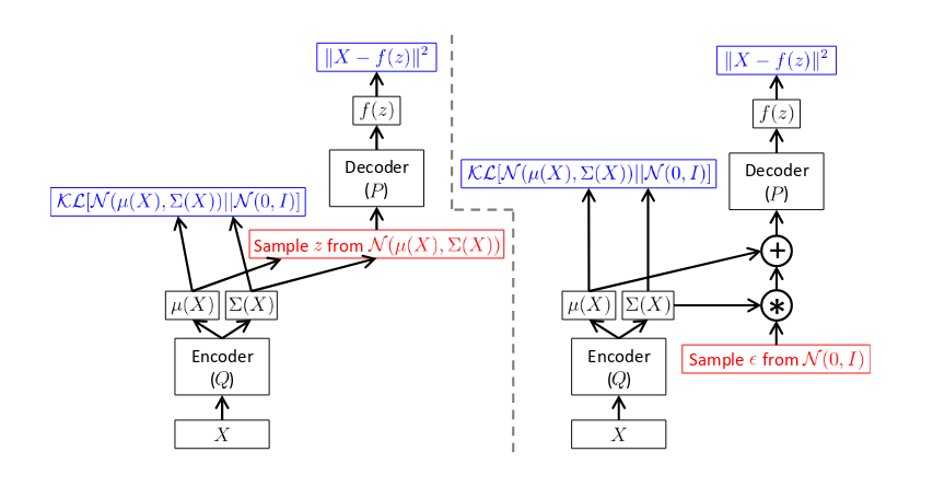
There is, however, a caveat. The network is not trainable using backpropagation because the red box is a stochastic step, which means that it is not differentiable. To solve this problem, we use the reparametrization trick as follows.

After this trick, we get the final network as shown in the right in the above figure. Furthermore, we must have $\mathcal{D}_{KL}[Q(z\vert X)\vert \vert P(z\vert X)]$ approximately equal $0$ in the LHS. Since we have taken $Q$ to be a Gaussian, this means that the original density function $f$ should be such that $P(z\vert X)$ is a Gaussian. It turns out that such a function, which maximizes $P(X)$ and satisfies the said criteria, provably exists.

Although VAEs have strong theoretical support, they do not work very well in practice, especially in problems such as face generation. This is because the loss function used for training is log-likelihood, which ultimately leads to fuzzy face images which have high match with several $X$. Instead of using likelihood, we use the power of discriminative deep learning, which is where GANs come into the picture.

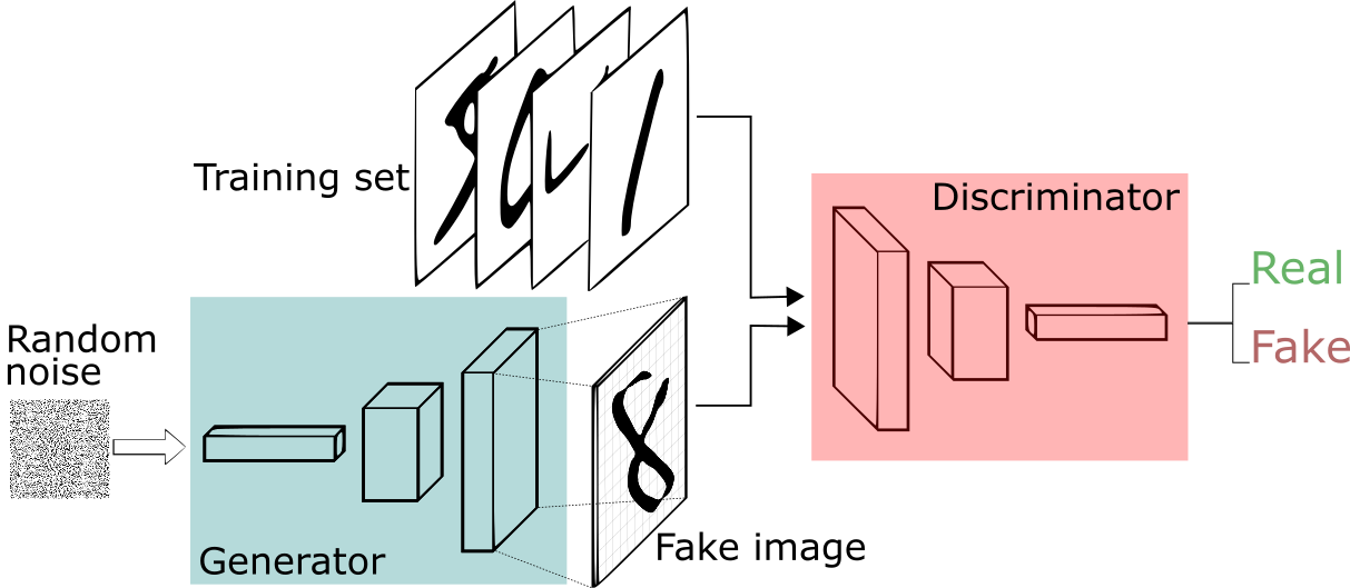
Generative adversarial networks: new insights

GANs were proposed in 2014, and have become immensely popular in computer vision ever since. They are basically motivated from game theory, and I will not get into the details here since the tutorial by Ian Goodfellow is a excellent resource for the same.

Since the prior learnt by the generator depends upon the discriminative process, an important issue with GANs is that of mode collapse. The problem is that since the discriminator only learns from a few samples, it may be unable to teach the generator to produce $\mathcal{P}_{synth}$ with sufficiently large diversity. In the context of what we have already seen, this can be taken as the problem of generalization for GANs.

In this section, I will discuss three results from two important papers from Arora et al. which deal with mode collapse in GANs.

• Generalization and equilibrium in generative adversarial nets
• Do GANs learn the distribution? Some theory and empirics

For all our discussions in this section, we will consider the Wasserstein GAN objective instead of the usual minimax objective, which is as follows (and arguably more intuitive)

where $D$ is the discriminator.

1. Generalization depends on discriminator size

If the discriminator size is $n$, then there exists a generator supported on $\mathcal{O}(n\log n)$ images, which wins against all possible discriminators.

This means that if we have a discriminator of size $n$, then the best possible generator training is possible using $Cn/\epsilon^2 \log n$ images from the full training set. Any more images will improve the training objective by at most $\epsilon$. I will now give the proof (simplified from the actual proof in the paper).

Proof: Suppose $\mu$ denotes the actual distribution learnt by the generator and $\nu$ denotes the actual distribution of real images that the discriminator has access to. Let $\tilde{\mu}$ and $\tilde{\nu}$ be the empirical versions of the above distributions, i.e., the distributions that we actually use for training. Let $d(p,q)$ be some distance measure between the two distributions.

In the paper, the authors have defined an $\mathcal{F}$-distance that has good generalization properties, but I will not get into the details of that here for sake of simplicity. For this discussion, just assume that the distance measure is $d$. From my earlier post on generalization error in supervised learning, we say that a model generalizes well when, for some $\epsilon$,

Here, we don’t really know the error, but we can use our distance measure to the same effect. If the size of discriminator is $p$, we want to compute the sample complexity $m$ in terms of $p$ and $\epsilon$ such that the GAN generalizes. For that, we need a few approximations.

First we approximate the parameter space $\mathcal{V}$ using its $\frac{\epsilon}{8}$-net $\mathcal{X}$. This means that for every $\nu \in \mathcal{V}$, we can find a $\nu^{\prime}\in \mathcal{X}$ which is at a distance of at most $\frac{\epsilon}{8}$ from it. Assuming that the function computed by the discriminator $D$ is 1-Lipschitz, we can then say that $\lvert \mathbb{E}{x \sim \mu} D{\nu}(x) - \mathbb{E}{x \sim \mu} D{\nu^{\prime}}(x) \rvert \leq \frac{\epsilon}{8}$.

The $\epsilon$-net is taken so that we can apply concentration inequalities in this continuous finite space. You can read more about them here. Now, we can use Hoeffding’s inequality to bound the difference between true and empirical errors on this space as

Taking union bound over all $p$ parameters, we get that when $m \geq \frac{Cp\log (p/\epsilon)}{\epsilon^2}$, then the bound holds with high probability. Note that this sample complexity is $m = \mathcal{p\log p}$, which is what we wanted. Now we just need to show that this bound implies that the generalization error is bounded. Since we have taken the $\frac{\epsilon}{8}$-net approximation, we translate both the parameters in $\mathcal{X}$ back to $\mathcal{V}$, paying a cost of $\frac{\epsilon}{8}$ for each. Finally, we get, for every $D$,

We can prove a similar upper bound for $\nu$. Finally, with similar approximation arguments, and from the definition of our distance function, we get the desired result.

2. Existence of equilibrium

For GANs to be successful, they must find an equilibrium in the G-D game where the generator wins. In the context of the minimax equation, this means that switching min and max in the objective should not cause any change in the equilibrium. In the paper, the authors prove an $\epsilon$-approximate equilibrium, i.e., one where such a switching affects the expression by at most $\epsilon$.

If a generator net is able to generate a Gaussian distribution, then there exists an $\epsilon$-approximate equilibrium where the generator has capacity $\mathcal{O}(n\log n / \epsilon^2)$.

The proof of this result lies in a classical result in statistics, which says that any probability distribution can be approximated by a mixture of infinite Gaussians. For this, we just need to take the standard Gaussian $P(x)\mathcal{N}(x,\sigma^2)$ at every $x \in \mathcal{X}$ such that $\sigma^2 \rightarrow 0$, and take the mixture of all such Gaussians. The remaining proof is similar to the one done for the previous result, so I will not repeat it here.

3. Empirically detecting mode collapse

We have already seen that GAN training can be successful even if the generator has not learnt a good enough distribution, if the discriminator is small. But suppose we take a really large discriminator and then train our GAN to a minima. How do we still make sure that the generator distribution is good? It could well be the case that the generator has simply memorized the training data, due to which the discriminator cannot make a better guess than random. Researchers have proposed several qualitative checks to test this:

• Check the similarity of each generated image to the nearest image in the training set.
• If the seed formed by interpolating two seeds $s_1$ and $s_2$ that produce realistic images, also produces realistic images, then the learnt distribution probably has many realistic images.
• Check for semantically important directions in latent space, which cause predictable changes in generated image.

We will now see a new empirical measure for the support size of the trained distribution, based on the Birthday Paradox.

The birthday paradox

In a room of just 23 people, there’s a 50% chance of finding 2 people who share their birthday.

To see why, refer to this post. It is a simple problem of permutation and combination, followed by using the approximation for $e^x$.

Since $23 \approx \sqrt{365}$, we can generalize this to mean that if a distribution has support $N$, we are likely to find a duplicate in a batch of about $\sqrt{N}$ samples taken from this distribution. As such, finding the smallest batch size $s$ which ensures duplicate images with good probability almost guarantees that the distribution has support $s^2$. Let us formalize this guarantee.

Suppose we have a probability distribution $P$ on a set $\Omega$. Also, let $S \subset \Omega$ such that $\sum_{s\in S}P(s)\geq \rho$ and $\vert S\vert=N$. Then from calculations similar to the one done for birthday paradox, we can say that the probability of finding at least one collision on drawing $M$ i.i.d samples is at least $1 - \exp\left( -\frac{(M^2 - M)\rho}{2N} \right)$.

Now, suppose we have empirically found this minimum probability of collision to be $\gamma$. Then it can be shown that under realistic assumptions on parameters, the following holds:

This gives an upper bound on the support size of the distribution learned by the generator.

Generative models are definitely very promising, especially with the recent interest in transfer learning with unsupervised pretraining. While I have tried to explain the recent insights into GANs as best as possible, it is not possible to explain every detail in the proof in an overview post. Even so, I hope I have been able to at least give a flavor of how veterans in the field approach theoretical guarantees.