Online Learning of Word Embeddings

Word vectors have become the building blocks for all natural language processing systems. I have earlier written an overview of popular algorithms for learning word embeddings here. One limitation with all these methods (namely SVD, skip-gram, and GloVe) is that they are all “batch” techniques. In this post, I will discuss two recent papers (which are very similar but were developed independently) which aim to provide an online approximation for the skip-gram algorithm.

But first, what do we mean by a “batch” algorithm?

Simply put, in a batch algorithm, the entire data set needs to be available before we begin the processing. In contrast, an “online” algorithm can process inputs on-the-fly, i.e., in a streaming fashion. Needless to say, such algorithms are also preferable when the available resources are not sufficient to process the entire dataset at once.

Now that we have some idea about batch algorithms, I’ll explain why the existing methods for word representation learning are of this kind. First, in the case of the standard SVD and Stanford’s GloVe, the entire cooccurence matrix needs to be computed, and only then can the processing be started. If some additional data arrives later, the matrix would have to be recomputed, and training would have to be restarted (if at least one of the updates depends on a changed matrix element). Second, in the case of Mikolov’s word2vec (skip-gram and CBOW), negative sampling is often used to make the computation more efficient. This sampling depends on the unigram probability distribution of the vocabulary words in the corpus. As such, before learning can happen, we need to compute the vocabulary as well as the unigram distribution.

Recently, two very similar methods (developed independently) have been proposed to make the skip-gram with negative sampling (SGNS) algorithm learn in a streaming fashion. I’ll quickly review the SGNS algorithm first so that there is some context when we discuss the papers.

Batch SGNS algorithm

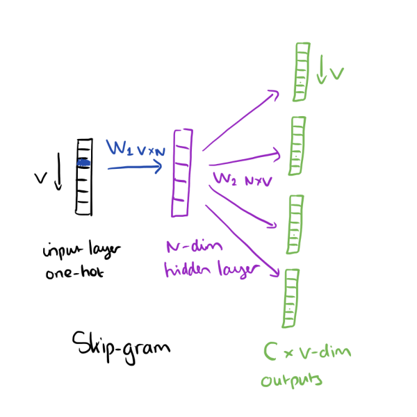
The above image is taken from The Morning Paper.

SGNS is a window-based method with the following training objective: Given the target word, predict all the context words in the window.

Suppose we have a context window where $w$ is the target word and $c$ is one of the context words. Then, skip-gram’s objective is to compute $P(c\vert w)$, which is given as

Basically, it is just a softmax probability distribution over all the word-context pairs in the corpus, directed by the cosine similarity. However, the denominator term here is very expensive to compute since there may be a very large number of possible context words. To solve this problem, negative sampling is used.

Goldberg and Levy have explained the derivation for the objective function in SGNS very clearly in their note. I will try to provide a little intuition here.

For the word $w$, we are trying to predict the context word $c$. Since we are using softmax, this is essentially like a multi-class classification problem, where we are trying to classify the next word into one of $N$ classes (where $N$ is the number of words in the dictionary). Since $N$ may be quite large, this is a very difficult problem.

What SGNS does is that it converts this multi-classification problem into binary classification. The new objective is to predict, for any given word-context pair $(w,c)$, whether the pair is in the window or not. For this, we try to increase the probability of a “positive” pair $(w,c)$, while at the same time reducing the probability of $k$ randomly chosen “negative samples” $(w,s)$ where $s$ is a word not found in $w$’s context. This leads to the following objective function which we try to maximize in SGNS:

In other words, we push the target vector in the direction of the positive context vector, and pull it away from $k$ randomly chosen (w.r.t. the unigram probability distribution) negative vectors. Here “negative” means that these vectors are not actually present in the target’s context.

What do we need to make SGNS online?

As is evident from the above discussion, since SGNS is a window-based approach, the training itself is very much in an online paradigm. However, the constraints are in creating a vocabulary and a unigram distribution for negative sampling, which makes SGNS a two-pass method. Further, if additional data is seen later, the distribution and vocabulary would change, and the model would have to be retrained.

Essentially, we need online alternatives for 2 aspects of the algorithms:

1. Dynamic vocabulary building
2. Adaptive unigram distribution

With this background, I will now discuss the two proposed methods for online SGNS.

Space-Saving word2vec

In this paper¹ from researchers at Johns Hopkins, the following solutions were proposed for the two problems mentioned above.

1. Space-saving algorithm for dynamic vocabulary building.
2. Reservoir sampling for adaptive unigram distribution.

Space-saving algorithm: It is a popular method to estimate the top-$k$ most frequent items in a streaming data.

• We declare a structure V containing $k$ pairs of word and their counts, and initialize it to empty pairs.
• As word $w$ arrives, if $w \in V$, we increment its count.
• Otherwise, if $V$ has space, we append the pair $(w,1)$ to $V$.
• If not, the word with the lowest count is replaced by $w$.

At any instant, the words in the structure V denote the dynamic vocabulary of the corpus.

Reservoir sampling: Reservoir sampling is a family of randomized algorithms for randomly choosing a sample of $k$ items from a list S containing $n$ items, where $n$ is either a very large or unknown number. (Wikipedia)

• Similar to the SS algorithm, we declare a structure (called the reservoir) of $k$ empty elements (not pairs this time). In addition, we initialize a counter $c$ to 0.
• The first $k$ elements in the stream are filled into the reservoir. $c$ is incremented at every occurence.
• For the remaining items, we draw $j$ from $1,\ldots,c$ randomly. If $j < k$, the $j^{\text{th}}$ element of the reservoir is replaced with the new element.

At any instant, the samples present in the reservoir provide an approximate distribution of items in the entire data stream.

While the algorithm itslelf is conceptually simple, the authors have mentioned several implementation choices which are important for training SGNS online. I list them here with some observations:

1. When a word is ejected from a bin in the dynamic vocabulary, its embeddings are re-initialized. As such, every bin has its own learning rate which is reset when the word in the bin is changed.
2. During sentence subsampling, all words not in $W$ are retained. Those in $W$ are retained with a probability which is inversely proportional to the square root of its count in the dictionary.
3. Probably the most important deviation from the SGNS algorithm is that the reservoir sampling essentially generates an empirical distribution from which to sample negative context words. In contrast, in the original SGNS algorithm, a smoothed empirical distribution is used. The authors have themselves allowed that “ smoothing the negative sampling distribution was (sic) shown to increase word embedding quality consistently.”

Incremental SGNS

This EMNLP’17 paper² from researchers at Yahoo Japan proposes the following alternative solutions for the aforementioned problems.

1. Misra-Gries algorithm for dynamic vocabulary building.
2. A modified reservoir sampling algorithm for adaptive unigram table.

Misra-Gries algorithm: This was developed long before the space-saving algorithm (1982) and was the go-to technique for top-$k$ most frequent itemset estimation in streaming data, before the space-saving algorithm was developed. The method is very similar to SS except for one difference:

• When word $w$ is not in $V$ and there is no space to append, every element in $V$ is decremented until some element becomes 0, at which point it is replaced by the new word.

Modified reservoir sampling: Here is the pseudocode from the paper.

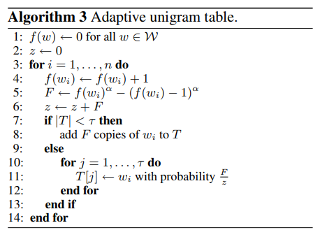
This algorithm differs from the conventional Reservoir Sampling in two important ways:

1. The counts used here are smoothed (see line 4 to 6). This has been shown to be important for word vector quality, as discussed above.
2. If the reservoir does not have enough space, we iterate over all existing words and replace them with some probability (which is proportional to the smoothed count of $w$). Contrast this with the earlier technique, where a $j$ was randomly sampled and word at that index was replaced. (Disclaimer: I am not sure how exactly this modification helps in learning. If I am allowed to venture a guess, I would say that it is a “soft” equivalent of the hard replacement in the original algorithm. This probably helps in the theoretical analysis of the algorithm.)

In addition, the authors have also provided theoretical justification for their algorithm and proved the following theorem: The loss in case of incremental SGNS converges in probability to that of batch SGNS.

In summary, SGNS is probably the easiest batch word embedding algorithm to “streamify” because of its inherent window-based nature. The constraints of vocabulary and counts are addressed with approximation algorithms. I can think of several possible directions in which this work can be continued.

First, there are several algorithms for estimating the top-$k$ most frequent items in a data stream. These are divided into count-based and sketch-based methods. The SS algorithm is probably the most efficient count-based technique, but it may be useful to look at other methods to see if they provide some edge. (Although I’m pretty sure the JHU researchers would have been thorough in their selection of the algorithm.)

Second, GloVe and SVD are yet to be addressed. In case of GloVe in particular, the problem would be to construct the co-occurence matrix in a online fashion. There should be some related work in statistics which can be leveraged for this, but I haven’t conducted much literature survey in this direction.