Sparsity in Online Learning with Lasso Regularization

Sparse vectors have become popular recently for 2 reasons:

1. Sparse matrices require much less storage since they can be stored using various space-saving methods.
2. Sparse vectors are much more interpretable than dense vectors. For instance, the non-zero non-negative components of a sparse word vector may be taken to denote the weights for certain features. In contrast, there is no interpretation for a value like $-0.1347$.

Sparsity is often induced through the use of L1 (or Lasso) regularization. There are 2 formulations of the Lasso: (i) convex constraint, and (ii) soft regularization.

Convex constraint

As the name suggests, a convex constraint is added to the minimization problem so that the parameters do not exceed a certain value.

The smaller the value of the tuning parameter $t$, fewer is the number of non-zero components in the solution.

Soft regularization

This is just the Lagrange form the the convex constraint, and is used because it is easier to optimize. Note that it is equivalent to the convex constraint formulation for an appropriately chosen $g$.

There is a great theoretical explanation of sparsity with Lasso regularization by Ryan Tibshirani and Larry Wasserman which you can find here. I will instead be focusing on some methods that have been introduced recently for inducing sparsity while learning online i.e., when the samples are obtained one at a time. In addition to such a scenario, online learning also comes into the picture when the data set is simply too large to be loaded in memory at once, and there are not sufficient resources for performing batch learning in a parallel fashion.

In this post, I will summarize 3 such methods:

1. Stochastic Truncated Gradient¹
2. Forward Backward Splitting²
3. Regularized Dual Averaging³

But first, why a simple soft Lasso regularization won’t work? With the soft regularization method, we are essentially summing up 2 floating point values. As such, it is highly improbable that the sum will be zero, since very few pairs of floats add up to zero.

Stochastic Truncated Gradient (STG)

STG combines ideas from 2 simple techniques:

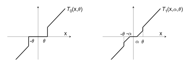
1. Coefficient rounding: In this method, the coefficients are rounded to 0 if they are less than a value $\theta$. This is denoted in the figure above (left graph). The rounding is done after every $k$ steps. The problem with this approach is that if $k$ is small, the coefficients do not get an opportunity to reach a value above $\theta$ before they are pulled back to $0$. On the other hand, if $k$ is large, the intermediate steps in the algorithm need to store a large number of non-zero coefficients, which does not solve the storage issue.
2. Sub-gradient method: In this method, L1-regularization is performed by shifting the update in the opposite direction depending on the sign of the coefficient. The update equation is

STG combines rounding from (1) and gravity from (2) so that (i) sparsity is achieved (unlike the sub-gradient method), and (ii) the rounding off is not too aggressive (unlike the direct rounding approach). The parameter update is then given by the function $T_1$ (shown in the right graph above).

The update rule is given using $T_1$ as

Here, $g$ may be called the gravity parameter, and $\theta$ is called the truncation parameter. In general, the larger these parameters are, the more sparsity is incurred. This can be understood easily from the definition of the truncation function.

Furthermore, note that on setting $\theta = \infty$ in the truncation function yields a special case of the Sub-gradient method wherein max and min operations are performed after applying gravity pull.

In the remainder of the paper, the authors prove a strong regret bound for the STG method, and also provide an efficient implementation for the same. Furthermore, they show the asymptotic solution of one instance of the algorithm is essentially equivalent to the Lasso regression, thus justifying the algorithm’s ability to produce sparse weight vectors when the number of features is intractably large.

Forward Backward Splitting (FOBOS)

Note: The method was named Forward Looking Subgradient (FOLOS) in the first draft and later renamed since it was essentially the same as an earlier proposed technique, the Forward Backward Splitting. The authors abbreviated it to FOBOS instead of FOBAS to avoid confusing readers of the first draft.

First, a little background. Consider an objective function of the form $f(w) + r(w)$. In the case of a number of machine learning algorithms, the function $f$ denotes the empirical sum of some loss function (such as mean squared error), and the function $r$ is a regularizer (such as Lasso). If we use a simple gradient descent technique to minimize this objective function, the iterates would be of the form

where the $g$’s are vectors from the subgradient sets of the corresponding functions. From the paper:

A common problem in subgradient methods is that if $r$ or $f$ is non-differentiable, the iterates of the subgradient method are very rarely at the points of non-differentiability. In the case of the Lasso regularization function, however, these points are often the true minima of the function.

In other words, the subgradient approach will result in neither a true minima nor a sparse solution if $r$ is the L1 regularizer.

FOBOS, as the name suggests, splits every iteration into 2 steps — a forward step and a backward step, instead of minimizing both $f$ and $r$ simultaneously. The motivation for the method is that for L1 regularization functions, true minima is usually attained at the points of non-differentiability. For example, in the 2-D space, the function resembles a Diamond shape and the minima is obtained at one of the corner points. Each iteration of FOBOS consists of the following 2 steps:

The first step is a simple unconstrained subgradient step with respect to the function $f$. In the second step, we try to achieve 2 objectives:

1. Stay close to the interim update vector. This is achieved by the first term.
2. Attain a low complexity value as expressed by $r$. (Second term)

So the first step is a forward step, where we update the coefficient in the direction of the subgradient, while the second is a backward step where we pull the update back a little so as to obtain sparsity by moving in the direction of the non-differentiable points of $r$.

Using the first equation in the second, taking derivative w.r.t $w$, and equating the derivative to $0$, we obtain the update scheme as

(Note: The equation above looks suspiciously similar to the Nesterov Accelerated Gradient (NAG) method for optimization. The authors have even cited Nesterov’s paper in related work. It might be interesting to investigate this further.)

This update scheme has 2 major advantages, according to the author.

First, from an algorithmic standpoint, it enables sparse solutions at virtually no additional computational cost. Second, the forward-looking gradient allows us to build on existing analyses and show that the resulting framework enjoys the formal convergence properties of many existing gradient-based and online convex programming algorithms.

In the paper, the authors also prove convergence of the method and show that on setting the intermediate learning rate properly, low regret bounds can be proved for both online as well as batch settings.

Regularized Dual Averaging (RDA)

Both of the above discussed techniques have one limitation — they perform updates depending only on the subgradients at a particular time step. In contrast, the RDA method “exploits the full regularization structure at each iteration.” Also, since the authors derive closed-form solutions for several popular optimization objectives, it follows that the computational complexity of such an approach is not worse than the methods which perform updates only based on current subgradients (both being $\mathcal{O}(n)$).

RDA comprises of 3 steps in every iteration.

In the first step, the subgradient is computed for that particular time step. This is the same as every other subgradient-based online optimization method.

The second step consists of computing a running average of all past subgradients. This is done using the online approach as

In the third step, the update is computed as

Let us try to understand this update scheme. First, the function $h(w)$ is a strongly convex function such that the update vector which minimizes it also minimizes the regularizer. In the case of Lasso regularization, $h(w)$ is chosen as follows.

where $\rho$ is a parameter called the sparsity enhancing parameter. $\beta$ is a predetermined non-negative and non-decreasing sequence.

Now to solve the equation, we can just take the derivative of the argument of argmin and equate it to $0$. On solving this equation, we get an update of the form

So the scheme ensures that the update is in the same convex space as the regularized dual average. Sparsity can further be controlled by tuning the value of the parameter $\rho$. The scaling factor can be regulated using the non-decreasing sequence selected at the beginning of the algorithm. For the case when it is equal to the time step $t$, the new coefficient is simply the sum of the dual average and the sparsity parameter.

The above is just my attempt at understanding the update scheme for RDA. I would be happy to discuss it further if you find something wrong with this explanation.

Now the method itself would become extremely infeasible if this differentiation would have to be performed for every iteration. However, for most commonly used regularizers and loss functions, the update rule can be represented with a closed-form solution. For this reason, the overall algorithm has the same complexity as earlier algorithms which use only the current step subgradient for performing updates.