These are my notes taken while reading the RLHF book by Nathan Lambert. Some of the sections are additionally based on other sources (these will be noted wherever appropriate).
The italicized text in indented block are some personal musings.
Table of Contents
- Introduction
- Definitions and background
- Training Overview
- Preference Data
- Reward Modeling
- Regularization
- Instruction tuning
- Rejection sampling
- Policy gradient algorithms
- Direct alignment
Introduction
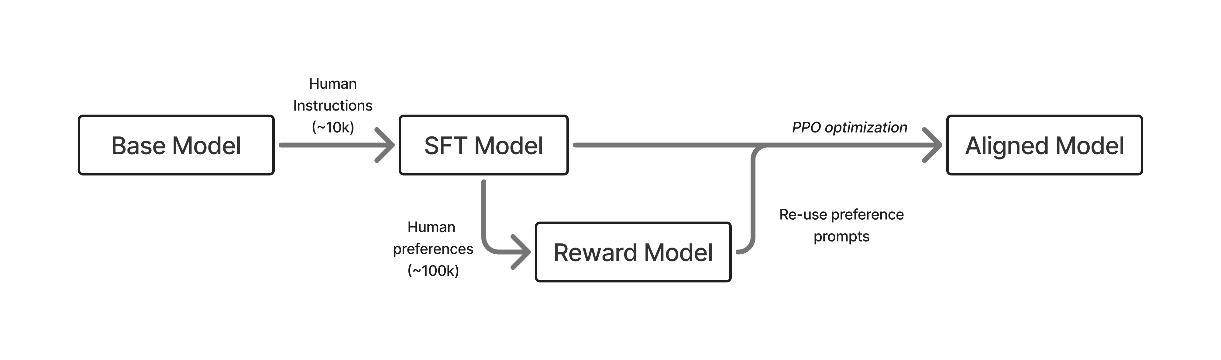
Basic pipeline of RLHF:
- Train an LM that can follow human questions.
- Collect human preference labels and train a reward model.
- Optimize the LM with an RL optimizer –> sample generations and rank them using the reward model
RL optimization requires an order of magnitude more prompts than SFT.
What does RLHF do?
- While SFT fine-tunes the model at the token level, RLHF tunes it at the response level.
- Additionally, it is telling the model what a “better” response should look like, rather than a specific response it should learn.
The elicitation interpretation of post-training
- Post-training is basically extracting and amplifying valuable behaviors in the base model. This is also called the “Superficial Alignment Hypothesis” in the LIMA paper.
- The base model has much more potential than what we can teach it simply by next token prediction (i.e., in SFT).
Some history
- RLHF first became popular with ChatGPT.
- After initial excitement, there were some naysayers who claimed that instruction fine-tuning is sufficient for alignment.
- IDPO became a work-horse especially for academic labs with smaller budgets.
- Around 2024, this idea was debunked as more labs published models with extensive post-training, including multiple rounds of SFT and RLHF (e.g. LLaMA 3.1).
Definitions and background
-
An autoregressive LM factorizes the probability of a sequence of tokens into a product of conditional probabilities: \(P_{\theta}(x) = \prod_{t=1}^{T} P_{\theta}(x_{t} \mid x_{1}, \ldots, x_{t-1})\)
- Here, $P_{\theta}$ is a neural network (such as a decoder-only Transformer) which is trained by minimizing the negative log-likelihood: \(\mathcal{L}_{\text{LM}}(\theta)=-\,\mathbb{E}_{x \sim \mathcal{D}}\left[\sum_{t=1}^{T}\log P_{\theta}\left(x_t \mid x_{<t}\right)\right]\)
- KL-divergence is a measure of the difference between two probability distributions:
\(D_{KL}(P \vert\vert Q) =
\sum_{x \in \mathcal{X}} P(x) \log \left(\frac{P(x)}{Q(x)}\right)\)
RL definitions
- Reward ($r$) is a scalar value indicating the desirability of a state or action.
- Action ($a$) is a move made by an agent among a set of possible moves, $A$.
- State ($s$) is the current configuration of the environment, where $S$ denotes state space.
- Trajectory: $\tau = (s_0,a_0,r_0,\ldots,s_T,a_T,r_T)$.
- Policy: ($\pi$) is a strategy that the agent follows to decide which action to take given a state.
- Discounting factor ($\gamma$) is exponential down-weighting of future rewards in the return.
- Value function is the estimated cumulative reward from a given state, i.e., \(V(s) = \mathbb{E}[\sum_{t=0}^{\infty} \gamma^t r_t \vert s_0 = s]\)
- Q-function estimates the expected cumulative reward from taking a specific action in a given state, i.e., \(Q(s,a) = \mathbb{E}[\sum_{t=0}^{\infty} \gamma^t r_t \vert s_0 = s, a_0 = a]\)
- Advantage function: $A(s,a) = Q(s,a) - V(s)$
- Policy-conditioned values: Data or values are often conditioned on the current policy, e.g. $V^\pi,A^\pi,Q^\pi$.
- The primary goal in RL is to maximize the expected cumulative reward: \(\max_{\theta} \mathbb{E}_{s \sim \rho_\pi, a \sim \pi_\theta}[\sum_{t=0}^{\infty} \gamma^t r_t]\)
- On-policy: In general RL, it means that data is generated by the current form of agent. In RLHF, it means that data is generated by the current edition of the model (v/s off-policy where the data can be from any other model or a previous edition of the current model).
Training Overview
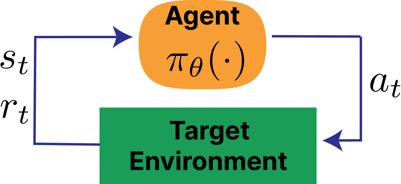
The standard RL loop looks like:
In contrast, the standard RLHF loops is as follows:
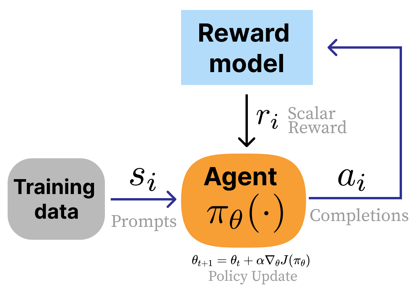
The main differences are:
- A reward model $r_{\theta}(s_t,a_t)$ is used which is a learned model of human preferences.
- There are no state transitions.
- Reward is on the entire completion, rather than for each token (this is often called a bandit problem).
The “HF” part of RLHF is because the reward model is trained on human feedbacks. Recently, alternatives such as RLAIF and RLVR have become popular. In RLAIF (“AI feedback”), the reward model is an off-the-shelf LLM. In RLVR (“verifiable rewards”), a verifier function checks the response, for example it can be running a Python code.
The overall loss function is as follows:
\[J(\pi) = \mathbb{E}_{\tau \sim \pi} \left[r_\theta(s_t, a_t)\right] - \beta \mathcal{D}_{KL}(\pi^{\text{RL}}(\cdot\vert s_t) \vert\vert \pi^{\text{ref}}(\cdot\vert s_t))\]Here, the KL-divergence term ensures that the model does not stray too far away from the strong SFT’d initialization.
Canonical recipes
InstructGPT This is the standard recipe which has become popular in several models.
- Instruction tuning on ~10k examples
- Train a reward model on ~100k prompts (pairwise preferences)
- Train the instruction-tuned model with RLHF on ~100k prompts
DeepSeek R1 This was specifically trained for reasoning first, followed by general queries.
- “Cold-start” of 100K on-policy reasoning samples
- Large-scale RLVR training
- Rejection sampling with 3:1 ratio of reasoning-to-general prompts
- Mixed RL with VR for reasoning and HF for general queries.
Preference Data
- Why do we need preference data?
- Because directly capturing human values in a reward function is impossible.
- It is much easier to collect pairwise (or ranked) labels for responses to the same prompt.
- Examples of bias in preference data
- Prefix bias
- Sycophancy
- Verbosity
- Formatting habits
- Rankings v/s ratings
- Most common technique is to use a 5-point Likert scale, i.e., A » B, A > B, tie, A < B, A « B
- Structured preference data
- It is created synthetically by prompting the model with and without constraint, or any other way that makes it easy to create positive and negative example.
- Alternatives
- Collect single datapoints with directional labels
- Use algorithms such as Kahneman-Tversk Optimization (KTO)
- There are also other algorithms to work with different types of feedback signals
*Also see paper on Step-KTO published by Meta authors.
Reward Modeling
- Bradley-Terry model of preferences measures the probability that the pairwise comparison for two events drawn from the same distribution satisfies the relation $i>j$: \(P(i>j) = \frac{p_i}{p_i+p_j}\)
- For prompt $x$ and responses $y_w$ and $y_l$, we can train a reward model for the above relation using the following loss: \(\mathcal{L}(\theta) = - \log \left( \sigma \left( r_{\theta}(x, y_w) - r_{\theta}(x, y_l) \right) \right)\)
- The most common way to train a reward model is to replace the final linear layer with a linear head that outputs regression scores. This is usually trained for just 1 epoch to avoid overfitting.
- LLaMA-2 proposed “preference margin loss”. If preference is provided on Likert scale, the extra information can be included in a margin term in the loss. This term was removed in LLaMA-3, however.
- If we have K-wise comparisons, we can use a modified loss function based on the Plackett-Luce model to train the RM.
- The traditional RM computes a reward for the whole sequence. There are also some variants:
- Outcome RM: It emits a reward per “token”, so it is modeled like an LM.
- Process RM: It emits a reward per “step” of a reasoning process.
- Generative reward models: Instead of training an RM, use LLM-as-judge. In such cases, the judge uses a temperature of 0 (i.e., greedy decoding) to reduce variance.
Here is an interesting paper about the theory behind Bradley-Terry models in RM, and a comprehensive survey about them.
Regularization
- We want to prevent over-optimization of the reward model.
- The most popular strategy is to add a KL-divergence term between the current model and the reference model to the optimization term: \(r = r_\theta - \lambda_{\text{KL}} \mathcal{D}_{\text{KL}} \left( \pi^{\text{RL}}(y \mid x) \, \vert\vert \, \pi^{\text{Ref.}}(y \mid x) \right)\)
- In practice, we compute the expected KL-divergence rather than the full-sum version, since it is much easier to implement.
- Another option, like that used in DPO, is to add a NLL-loss regularization to the objective.
- Regularization has not been used much in RM training, however.
Instruction tuning
- Even before GPT-3, many large text models were being developed (such as T-5, FLAN, etc.) with the idea of representing different NLP tasks in a common format and training a single large transformer for them.
- Instruction tuning (IFT) is the simplest way to adapt a pre-trained LLM for a desired task.
- In general, the data used for IFT is formatted to contain “system”, “user”, and “assistant” parts, where the loss is applied only on the last.
- Key differences from pre-training:
- Smaller batch sizes
- Prompt masking
- Multi-turn masking, i.e., train only on last-turn response
Rejection sampling
- In computational statistics, “rejection sampling” (RJS) is a way to sample from a complex distribution. To do this, we instead sample from a model distribution and use heuristics to check if the sample is permissible.
- In LLM post-training, RJS is used as follows:
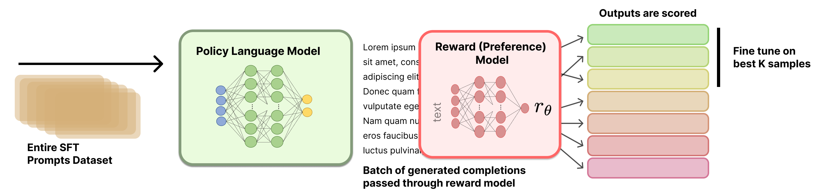
- How to select which prompt-response pairs to fine-tune? There are many options:
- Select top response per prompt
- Select top-K prompt-response pairs from the entire set
- Other details:
- Usually 10-30 completions are generated for each prompt
- Some implementations include generations from multiple models
- The RM used will heavily impact the final results
Policy gradient algorithms
Some of the notes in this section are based on a Meta-internal talk by Katerina Zmolikova.
General formulation
Suppose $\tau = (s_o,a_0,s_1,a_1,\ldots)$ is the trajectory and $R(\tau) = \sum_{t=0}^{\infty}r_t$ is the total reward of the trajectory. Then, the goal of the RL agent is to maximize the following objective:
\[J(\theta) = \mathbb{E}_{\tau \sim \pi_\theta} \left[ R(\tau) \right] = \int_{\tau}p_{\theta}(\tau)R(\tau)d\tau.\]In order to maximize this objective, we can take its gradient with respect to $\theta$:
\[\begin{align}\nabla_\theta J(\theta) &= \nabla_\theta \int_\tau p_\theta (\tau) R(\tau) d\tau \\ &=\int_{\tau} \nabla_\theta p_\theta (\tau) R(\tau) d\tau \quad \quad \text{(Leibniz rule)} \\ &= \int_{\tau} p_{\theta}(\tau) \frac{\nabla_\theta p_\theta(\tau)}{p_{\theta}(\tau)} R(\tau) d\tau \\ &= \int_{\tau} p_{\theta}(\tau) \nabla_{\theta}\log p_{\theta}(\tau) R(\tau) d\tau \quad \quad \text{(Log-derivative trick)} \\ &= \mathbb{E}_{\tau\sim \pi_{\theta}} [\nabla_{\theta}\log p_{\theta}(\tau)R(\tau)]. \end{align}\]The probability of the trajectory can be factorized as:
\[\begin{align} p_\theta (\tau) &= p(s_0) \prod_{t=0}^\infty \pi_\theta(a_t\vert s_t) p(s_{t+1}\vert s_t, a_t) \\ \implies \log p_\theta (\tau) &= \log p(s_0) + \sum_{t=0}^\infty \log \pi_\theta(a_t\vert s_t) + \sum_{t=0}^\infty \log p(s_{t+1}\vert s_t, a_t)\end{align}\]Taking the derivative of this w.r.t. $\theta$, we get:
\[\nabla_\theta \log p_{\theta}(\tau) = \underbrace{\nabla_\theta\log p(s_0)}_{\text{= 0}} + \nabla_\theta \sum_{t=0}^\infty \log \pi_\theta(a_t\vert s_t) + \underbrace{\nabla_\theta\sum_{t=0}^\infty \log p(s_{t+1}\vert s_t, a_t)}_{\text{= 0}}.\]Here, the first term is 0 since initial state does not depend on $\theta$, and the final term is 0 since transition dynamics don’t depend on $\theta$. Substituting the remainder term into the gradient of the objective:
\[\nabla_\theta J(\theta) = \mathbb{E}_{\tau\sim \pi_{\theta}}[\sum_{t=0}^{\infty}\nabla_\theta \log \pi_{\theta}(a_t\vert s_t)R(\tau)].\]In the above equation,
\[R(\tau) = \sum_{t=0}^{\infty}r_t.\]However, at any timestep $t$, the action $a_t$ can only influence the future rewards:
\[\begin{align}G_t &= R_{t+1} + \gamma R_{t+2} + \cdots = \sum_{k=o}^\infty \gamma^k R_{t+k+1}\\ &=\gamma G_{t+1} + R_{t+1}.\end{align}\]So, we can rewrite the gradient as:
\[\nabla_\theta J(\theta) = \mathbb{E}_{\tau\sim \pi_{\theta}}[\sum_{t=0}^{\infty}\nabla_\theta \log \pi_{\theta}(a_t\vert s_t)G_t].\]All of the policy gradient algorithms used in practice are based on variations of this gradient formulation.
Training algorithm
The training algorithm does the following in each iteration:
- Sample trajectories from current policy model.
- Compute rewards for each time step.
- Compute policy loss $-\sum_t \log \pi_{\theta}(a_t)R(\tau)$.
- Run backward step.
The important thing to note here is that in the actual training, we are optimizing a policy loss which just happens to have the same gradient as our actual objective $J(\theta)$. The value of this loss function is meaningless; it does not even need to go down during training.
REINFORCE
The naive gradient above has a large variance. In practice, it is better to only compute the advantage of the policy at the current state, i.e.,
\[A_t = G_t - b,\]and the resulting gradient is obtained as
\[\nabla_\theta J(\theta) = \mathbb{E}_{\tau\sim \pi_{\theta}}[\sum_{t=0}^{\infty}\nabla_\theta \log \pi_{\theta}(a_t\vert s_t)A_t].\]In practice, the “baseline” can be computed using a different value model, which is also updated at each time step.
Proximal policy optimization (PPO)
PPO does two additional things on top of the gradient formulation in REINFORCE.
Importance sampling
- In the original algorithm, we spend a lot of effort for each training step: sampling multiple trajectories, computing the rewards for all of them, computing value loss, etc.
- This is very inefficient use of data.
- To avoid this, PPO does multiple updates in each iteration without re-computing the trajectories and rewards. The problem with doing this naively is that this makes the updates “off-policy”, i.e., the data is sampled from an older policy model.
- To resolve this issue, we use importance sampling:
- Applying this to our problem, we get:
NOTE: The approximation in the second step has bounded difference. But this is the first time that the gradient is not exactly the gradient of the estimated reward!
Again, during training, we don’t compute the gradient directly. Instead, we just scale the policy loss by the importance sampling ratio above.
Clipping
- Large steps can be harmful in RL. PPO uses clipping to prevent this. The main change is:
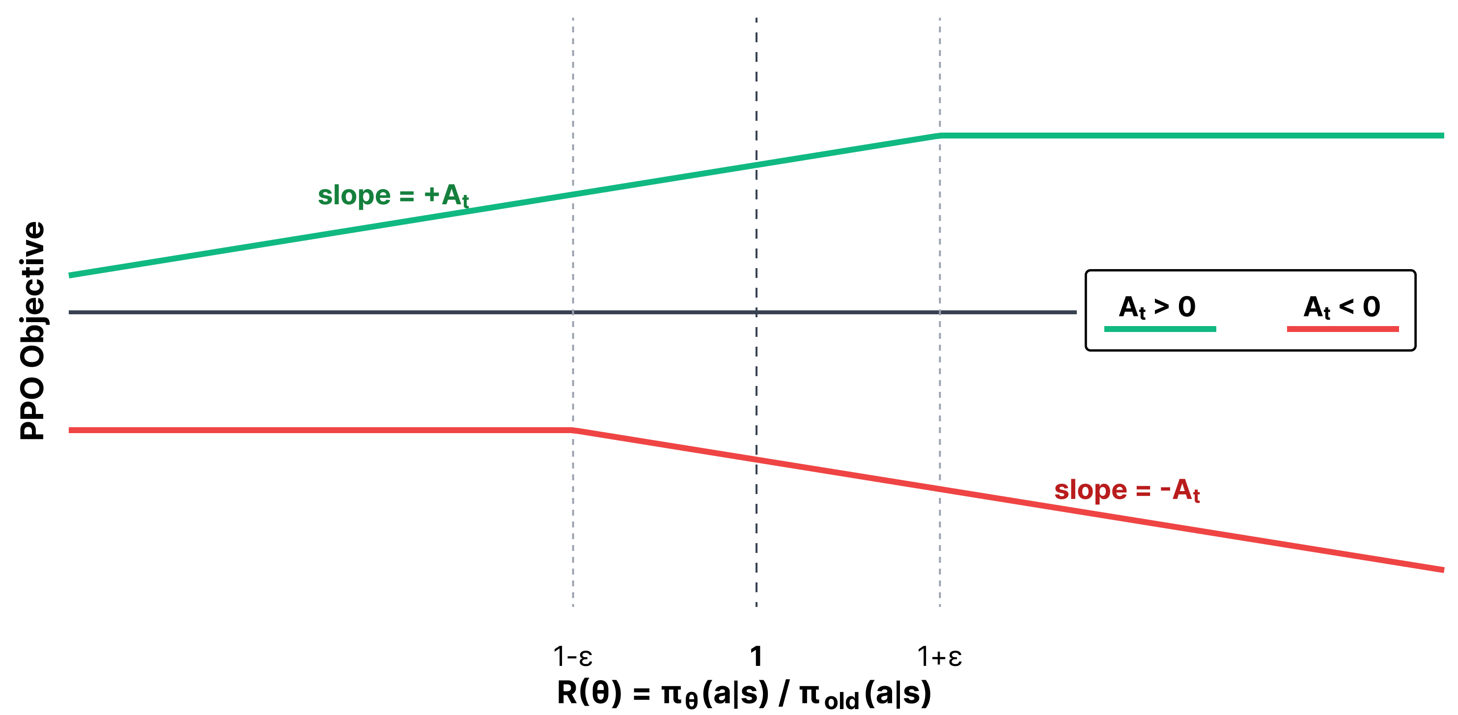
The above figure explains how the PPO objective works with clipping. The table below lists all the scenarios:
| Advantage | Meaning | $R(\theta) < 1-\epsilon$ | $1-\epsilon <= R(\theta) <= 1+\epsilon$ | $R(\theta) > 1+\epsilon$ |
|---|---|---|---|---|
| $A_t > 0$ | Action was beneficial | Normal update | Normal update | No update |
| $A_t < 0$ | Action was harmful | No update | Normal update | Normal update |
During RL, we usually also add KL-regularization to the loss to ensure that it doesn’t deviate too much from the base policy model. So overall, we need to keep 4 models in memory:
- policy model
- reward model
- value model
- reference model
REINFORCE Leave One Out (RLOO)
Do we really need all the fancy techniques in PPO when using RL on LLMs? The authors found that:
- We don’t need fancy variance reduction techniques.
- The baseline for advantage computation can be done by simple leave-one-out averaging rather than using an external value model.
- Removing clipping does not hurt performance.
- We can model entire completion as a single action (instead of computing reward per token).
Finally, the RLOO objective is:
\[\mathbb{E}_{\tau \sim \tau_{\theta}}\left[ \nabla_{\theta} \log \pi_{\theta}(a_t)(R-b(s)) \right],\]where
\[b(s, a_k) = \frac{1}{K-1}\sum_{i=1, i\neq k}^{K} R(s, a_i)\]Group Relative Policy Optimization (GRPO)
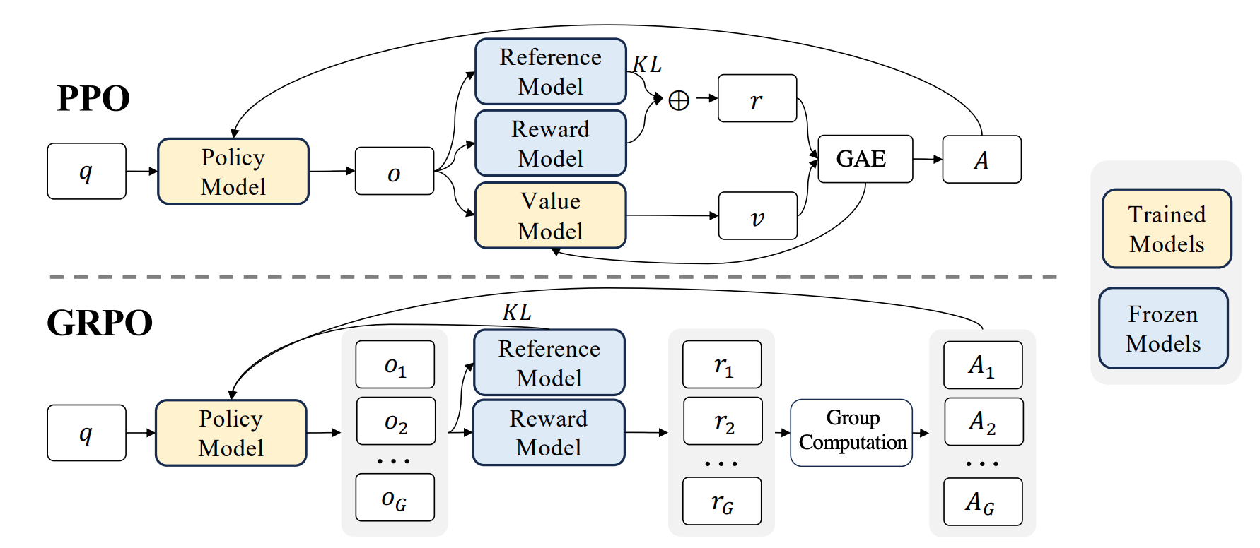
- Similar to RLOO, there is no separate Value model.
- Advantage is computed as:
- This normalization by std breaks the math, i.e., the gradient is no longer equal to the desired gradient.
- Another change is that the KL-divergence is directly included in the loss computation.
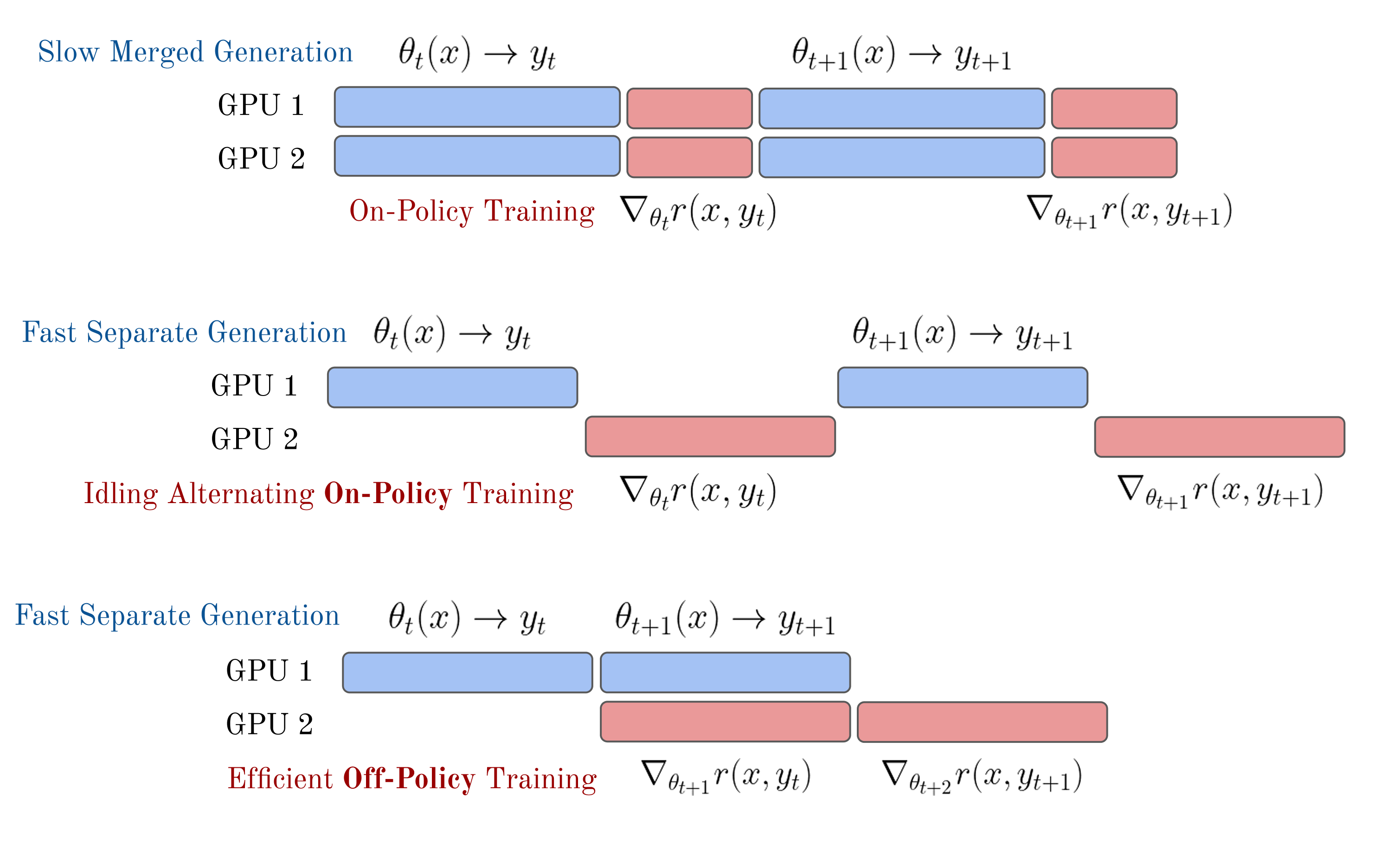
Implementation details
- Truly on-policy training will be slow since the trainer would need to wait for all inference to finish.
- To make training more efficient, training and inference are run asynchronously on separate GPUs, with the assumption that slightly off-policy data is okay.
Direct alignment
- While policy gradient methods work well, they need an intermediate reward model (RM) to be trained.
- Direct alignment methods seek to optimize the policy directly based on training data, without the need for RMs.
- The most prominent method in this category is DPO (Direct Preference Optimization).
Direct preference optimization (DPO)
This section is largely based on this blog post.
Suppose we have a collection of preference data $\mathcal{D}(\mathbf{x}^{(i)}, \mathbf{y}{w}^{(i)}, \mathbf{y}{l}^{(i)})$. We want to perform a kind of sequence discriminative training of our LLM, i.e., train it to generate responses which are closer to the winning samples than the losing samples.
Under the Bradley-Terry model, we want to model the true probability of human preferences as
\[p^{\ast}(i \succ j) = \frac{s_i}{s_i + s_j} = \sigma(r_i^{\ast} - r_j^{\ast}).\]The above is assuming that the “score” is parameterized as $s_i = e^{r_i}$.
In the context of our LLM, we want the following to be true:
\[p^{\ast}(\mathbf{y}_1 \succ \mathbf{y}_2 \vert \mathbf{x}) = \sigma(r^{\ast}(\mathbf{x},\mathbf{y}_1)-r^{\ast}(\mathbf{x},\mathbf{y}_2)).\]In the regular RLHF framework, we do this by learning a reward model $r_{\theta}$ using the following loss function,
\[\mathcal{L}_{R}(r_{\theta},\mathcal{D}) = -\mathbb{E}_{(\mathbf{x},\mathbf{y}_w,\mathbf{y}_l)}\left[\log \left(\sigma(r_{\theta}(\mathbf{x},\mathbf{y}_w)-r_{\theta}(\mathbf{x},\mathbf{y}_l))\right)\right]\]and then using the learned RM for policy gradient training.
However, in DPO, instead of this two-stage process, the idea is to optimize the policy model directly such that the above requirement is met. Suppose $\mathbf{r}(\mathbf{x},\mathbf{y})$ is some reward model. Then our goal is to maximize the expected reward while making sure that the model does not stray too far from the instruction-tuned base.
Let us write this out formally:
\[\begin{align} &\max_{\theta} \mathbb{E}_{\mathbf{y}\sim \pi_{\theta}(\mathbf{y}\vert \mathbf{x})}[\mathbf{r}(\mathbf{x},\mathbf{y})]-\beta~\mathbb{D}_{KL}[\pi_{\theta}(\mathbf{y}\vert \mathbf{x})\vert\vert \pi_{\text{ref}}(\mathbf{y}\vert \mathbf{x})] \\ =& \max_{\theta} \mathbb{E}_{\mathbf{y}\sim \pi_{\theta}(\mathbf{y}\vert \mathbf{x})}[\mathbf{r}(\mathbf{x},\mathbf{y})]-\beta~\mathbb{E}_{\pi_{\theta}(\mathbf{y}\vert \mathbf{x})}[\log\frac{\pi_{\theta}(\mathbf{y}\vert \mathbf{x})}{\pi_{\text{ref}}(\mathbf{y}\vert \mathbf{x})}] \\ =& \max_{\theta} \mathbb{E}_{\mathbf{y}\sim \pi_{\theta}(\mathbf{y}\vert \mathbf{x})}\left[\mathbf{r}(\mathbf{x},\mathbf{y})-\beta~\log\frac{\pi_{\theta}(\mathbf{y}\vert \mathbf{x})}{\pi_{\text{ref}}(\mathbf{y}\vert \mathbf{x})}\right] \\ =& \min_{\theta} \mathbb{E}_{\mathbf{y}\sim \pi_{\theta}(\mathbf{y}\vert \mathbf{x})}\left[\log\frac{\pi_{\theta}(\mathbf{y}\vert \mathbf{x})}{\pi_{\text{ref}}(\mathbf{y}\vert \mathbf{x})}-\frac{1}{\beta}\mathbf{r}(\mathbf{x},\mathbf{y})\right] \\ =& \min_{\theta} \mathbb{E}_{\mathbf{y}\sim \pi_{\theta}(\mathbf{y}\vert \mathbf{x})}\left[\log\pi_{\theta}(\mathbf{y}\vert \mathbf{x})-\log\pi_{\text{ref}}(\mathbf{y}\vert \mathbf{x})-\frac{1}{\beta}\mathbf{r}(\mathbf{x},\mathbf{y})\right] \\ =& \min_{\theta} \mathbb{E}_{\mathbf{y}\sim \pi_{\theta}(\mathbf{y}\vert \mathbf{x})}\left[\log\pi_{\theta}(\mathbf{y}\vert \mathbf{x})-\log\pi_{\text{ref}}(\mathbf{y}\vert \mathbf{x})-\log \exp\frac{1}{\beta}\mathbf{r}(\mathbf{x},\mathbf{y})\right] \\ =& \min_{\theta} \mathbb{E}_{\mathbf{y}\sim \pi_{\theta}(\mathbf{y}\vert \mathbf{x})}\left[\log\pi_{\theta}(\mathbf{y}\vert \mathbf{x})-\log\pi_{\text{ref}}(\mathbf{y}\vert \mathbf{x}) \exp\frac{1}{\beta}\mathbf{r}(\mathbf{x},\mathbf{y})\right] \\ =& \min_{\theta} \mathbb{E}_{\mathbf{y}\sim \pi_{\theta}(\mathbf{y}\vert \mathbf{x})}\left[\log\frac{\pi_{\theta}(\mathbf{y}\vert \mathbf{x})}{\pi_{\text{ref}}(\mathbf{y}\vert \mathbf{x}) \text{e}^{\frac{1}{\beta}\mathbf{r}(\mathbf{x},\mathbf{y})}}\right] \\ \end{align}\]So far, we have only done basic simplification using the definition of KL divergence and then combining the RM term. At this point, this would again resemble a KL divergence term, except that the denominator is not a probability distribution anymore. Well, let’s just make it a distribution but renormalizing it. Let
\[Z(\mathbf{x})=\sum_{\mathbf{y}}\pi_{\text{ref}}(\mathbf{y}\vert \mathbf{x}) \text{e}^{\frac{1}{\beta}\mathbf{r}(\mathbf{x},\mathbf{y})}.\]Then, we can divide both the numerator and denominator by $Z(\mathbf{x})$ as follows:
\[\begin{align} =& \min_{\theta} \mathbb{E}_{\mathbf{y}\sim \pi_{\theta}(\mathbf{y}\vert \mathbf{x})}\left[\log\frac{\frac{\pi_{\theta}(\mathbf{y}\vert \mathbf{x})}{Z(\mathbf{x})}}{\frac{\pi_{\text{ref}}(\mathbf{y}\vert \mathbf{x}) \text{e}^{\frac{1}{\beta}\mathbf{r}(\mathbf{x},\mathbf{y})}}{Z(\mathbf{x})}}\right] \\ =& \min_{\theta} \mathbb{E}_{\mathbf{y}\sim \pi_{\theta}(\mathbf{y}\vert \mathbf{x})}\left[\log\frac{\pi_{\theta}(\mathbf{y}\vert \mathbf{x})}{\frac{\pi_{\text{ref}}(\mathbf{y}\vert \mathbf{x}) \text{e}^{\frac{1}{\beta}\mathbf{r}(\mathbf{x},\mathbf{y})}}{Z(\mathbf{x})}}-\log Z(\mathbf{x})\right] \\ =& \min_{\theta} \mathbb{E}_{\mathbf{y}\sim \pi_{\theta}(\mathbf{y}\vert \mathbf{x})}\left[\log\frac{\pi_{\theta}(\mathbf{y}\vert \mathbf{x})}{\frac{\pi_{\text{ref}}(\mathbf{y}\vert \mathbf{x}) \text{e}^{\frac{1}{\beta}\mathbf{r}(\mathbf{x},\mathbf{y})}}{Z(\mathbf{x})}}-\log Z(\mathbf{x})\right] \\ \end{align}\]Now, since $Z(\mathbf{x})$ does not depend on $\pi_{\theta}$ or $\mathbf{y}$, we can completely ignore it from the above expectation term, giving us:
\[\begin{align} =& \min_{\theta} \mathbb{E}_{\mathbf{y}\sim \pi_{\theta}(\mathbf{y}\vert \mathbf{x})}\left[\log\frac{\pi_{\theta}(\mathbf{y}\vert \mathbf{x})}{\frac{\pi_{\text{ref}}(\mathbf{y}\vert \mathbf{x}) \text{e}^{\frac{1}{\beta}\mathbf{r}(\mathbf{x},\mathbf{y})}}{Z(\mathbf{x})}}\right]-\log Z(\mathbf{x}) \\ =& \min_{\theta} \mathbb{D}_{KL}\left[\pi_{\theta}(\mathbf{y}\vert \mathbf{x})\vert\vert\frac{1}{Z(\mathbf{x})}\pi_{\text{ref}}(\mathbf{y}\vert \mathbf{x}) \text{e}^{\frac{1}{\beta}\mathbf{r}(\mathbf{x},\mathbf{y})}\right]-\log Z(\mathbf{x}) \\ \end{align}\]To derive the optimal solution for a given $\mathbf{x}$, we can simply ignore the normalization constant. Then, the KL-divergence would be minimized (at 0) if the distributions are identical, i.e.,
\[\pi^*(\mathbf{y}\vert \mathbf{x})=\frac{1}{Z(\mathbf{x})}\pi_{\text{ref}}(\mathbf{y}\vert \mathbf{x}) \text{e}^{\frac{1}{\beta}\mathbf{r}(\mathbf{x},\mathbf{y})}.\]Unfortunately, obtaining the above optimal solution requires computing $Z(\mathbf{x})$, which is intractable (summation over exponentially many sequences). The other minor inconvenience is that we don’t really want to train the reward model $\mathbf{r}(\mathbf{x},\mathbf{y})$ explicitly. Let us try to rearrange the above equation to write it in terms of the optimal reward model $\mathbf{r}^*(\mathbf{x},\mathbf{y})$ by taking log on both sides:
\[\begin{align} \log \pi^*(\mathbf{y}\vert \mathbf{x})&=-\log Z(\mathbf{x})+\log \pi_{\text{ref}}(\mathbf{y}\vert \mathbf{x}) +\frac{1}{\beta}\mathbf{r}^*(\mathbf{x},\mathbf{y}) \\ \mathbf{r}^*(\mathbf{x},\mathbf{y}) &= \beta \log \frac{\pi^*(\mathbf{y}\vert \mathbf{x})}{\pi_{\text{ref}}(\mathbf{y}\vert \mathbf{x})} + \beta \log Z(\mathbf{x}) \end{align}\]Let us substitute this in the Bradley-Terry model that we want to estimate:
\[\begin{align} p^{\ast}(\mathbf{y}_1 \succ \mathbf{y}_2 \vert \mathbf{x}) &= \sigma(r^{\ast}(\mathbf{x},\mathbf{y}_1)-r^{\ast}(\mathbf{x},\mathbf{y}_2)) \\ &= \sigma\left(\beta \log \frac{\pi^*(\mathbf{y}_1\vert \mathbf{x})}{\pi_{\text{ref}}(\mathbf{y}_1\vert \mathbf{x})} + \beta \log Z(\mathbf{x}) - \beta \log \frac{\pi^*(\mathbf{y}_2\vert \mathbf{x})}{\pi_{\text{ref}}(\mathbf{y}_2\vert \mathbf{x})} - \beta \log Z(\mathbf{x})\right) \\ &= \sigma\left(\beta \log \frac{\pi^*(\mathbf{y}_1\vert \mathbf{x})}{\pi_{\text{ref}}(\mathbf{y}_1\vert \mathbf{x})} - \beta \log \frac{\pi^*(\mathbf{y}_2\vert \mathbf{x})}{\pi_{\text{ref}}(\mathbf{y}_2\vert \mathbf{x})}\right) \\ \end{align}\]Conveniently, we are only left with tractable quantities. In order to learn the parameters of $\pi^*(\mathbf{y}_2\vert\mathbf{x})$ that maximize the above probability, we can use MLE on the following loss:
\[\mathcal{L}_{\text{DPO}} = -\mathbb{E}_{(\mathbf{x},\mathbf{y}_w,\mathbf{y}_l)\sim \mathcal{D}}\left[\sigma\left(\beta \log \frac{\pi^*(\mathbf{y}_w\vert \mathbf{x})}{\pi_{\text{ref}}(\mathbf{y}_w\vert \mathbf{x})} - \beta \log \frac{\pi^*(\mathbf{y}_l\vert \mathbf{x})}{\pi_{\text{ref}}(\mathbf{y}_l\vert \mathbf{x})}\right) \right].\]This converts the RL problem into a much simpler supervised learning problem!
Limitations of DPO
The global optimizer of DPO and RLHF is the same when:
- The Bradley-Terry model perfectly fits our preference data
- RLHF learns the optimal reward function
However, the above are very rarely true. Another issue is that deterministic preferences (i.e. $p(\mathbf{y}_1 \succ \mathbf{y}_2 \vert \mathbf{x})=1$) can push $\pi(\mathbf{y}_l\vert\mathbf{x})$ to 0 very quickly.