I attended the Speech and Audio in the Northeast (SANE) 2019 conference at Columbia University last Thursday, and in this post, I will try to summarize some of the invited talks that I found interesting and a few of the posters that I spent some time at. (If a talk or a poster does not feature here, that probably just means I don’t work in that field or I don’t have sufficient background to understand the work.)

Invited Talks
1. Brian Kingsbury (IBM)
There were 2 parts to the talk: 1. How to train large DNNs fast? 2. Estimating information flow in DNNs.
How to train large DNNs fast?
Dr. Kingsbury summarized some of his group’s recent work on data parallel algorithms ([paper 1] [paper 2]) for acoustic model training. They train windowed BLSTM acoustic models with a cross-entropy per frame objective. This can be done in the following ways:
- Synchronous Parallel SGD (SPSGD): This is the most naive way to parallelize the training process. The idea is to distribute the gradient computation among the worker processes, and then perform an all-reduce operation to average the gradients. However, such an algorithm would be constrained by the speed of the slowest worker, and it also incurs high communication cost.
- Asynchronous Parallel SGD (APSGD): A simple way of avoiding these problems is a framework where workers do not wait on each other. Instead, batches are assigned to workers from a parameter server, and then the gradients are pushed as soon as computation is done. Although this solves the straggler problem, it can lead to slow convergence due to staleness of gradients, and this problem increases with an increase in number of workers. Moreover, the parameter server itself can become a bottleneck.
- Asynchronous Decentralized Parallel SGD (ADPSGD): In this method, the parameter server bottleneck is removed entirely. Instead, the workers are connected in a ring topology, and each worker calculates the gradient, updates its weights, and averages the weights with its neighbor. This has been shown to have convergence guarantees as well. In the follow-up paper (submitted to ICASSP), they show that very large batch sizes (10k, IIRC) can be used with this technique, and so it makes more efficient use of GPU resources with less communication cost. However, this may lead to bad convergence of held-out loss, which necessitates the use of something called “linear warmup”.
- Hierarchical ADPSGD: This combines the previous method with knowledge of the architecture. Since the within-node bandwidth is high, use SPSGD, and for the inter-node communication, use ADPSGD. With these improvements, training time for the 2000h SWBD can be reduced from 192 hours to 5.2 hours, and batch size can be effectively increased from 256 to 8192 without loss in performance.
Although the authors have only tried this on BLSTM architectures for now, similar methods have been used for convolutional networks in vision, to the same effect. The group is also planning to use these techiques for faster training of end-to-end ASR systems, and those with transformers.
Estimating information flow in DNNs
There has been a lot of effort for understanding DNNs, and most of these fall into one of the following 4 categories:
- Structure of the loss landscape
- Wavelets and sparse coding
- Adversarial examples
- Information theory
This work falls into the last category, and the authors use the popular Information Bottleneck approach. In essence, we can think about DNNs as a means for learning representations ($T_l$ is the representation leart at the output of layer $l$ of a DNN) of the input $X$ which can be helpful to predict the output $Y$. To do a good prediction job, the DNN needs to maximize $I(T_l;Y)$. However, to generalize better to unseen inputs, it also needs to minimize $I(T_l;X)$.
Earlier efforts in this direction have always dealt with deterministic DNNs, and used binning to estimate $I(T_l;X)$. The hypothesis is that training comprises 2 stages: (i) fitting, where $I(T_l;Y)$ and $I(T_l;X)$ increase rapidly, and (ii) compression, where $I(T_l;X)$ decreases slowly.
However, this estimate is only valid for very small bins, which makes the computation expensive. Furthermore, the authors showed that the binning estimator actually measures the clustering of samples in $T_l$ and not $I(T_l;X)$ itself. This is because this latter quantity is constant or infinite in deterministic DNNs, so its measure is vacuous.
Instead, the authors propose a method called auxiliary noise DNN framework, which injects a Gaussian noise at every layer which is small enough such that the $T_l$ does not change much. The MI is then estimated as
\[I(X;T_l) = h(T_l) - \frac{1}{m}\sum_{i=1}^m h(T_l|X=x_i),\]where $X \sim Unif(\mathcal{X})$.
2. Karen Livescu (TTI-Chicago)
Prof. Livescu’s talk was about acoustic and acoustically-grounded word embeddings. Usually (in NLP), when we talk about word embeddings, they measure semantic similarity. Instead, what if we wanted embeddings that could measure acoustic similarity? Such embeddings could potentially be useful for many tasks such as spoken term detection, query by example, and even ASR.
There’s an important difference between regular word embeddings and acoustic word embeddings. With the former, you can just have a list of words in your vocabulary and a vector corresponding to each word. However, when words are spoken, they may sound different every time if the speaker varies, or even for the same speaker depending on words in context. Here is an overview of Prof. Livescu’s work in this domain:
-
Originally, they used a template-based approach, where they had a predetermined set of $m$ template vectors, and for each input word, they created an $m$-dimensional vector by taking the DTW distance between the word and each template.
-
Later, they experimented with using deep convolutional networks and recurrent neural networks for automatically learning features, and found that RNNs work better.
-
They also experimented with different loss functions, and concluded that a triplet loss outperformed the traditional cross-entropy loss. The loss essentially minimizes the Euclidean distance between vectors corresponding to different instances of the same word, and maximizes the distance between different words.
The second part of the talk was on “acoustically grounded embeddings”, which can be seen as a multi-view extension of acoustic embeddings, where we have the written instance in addition to the spoken instance. The key observation was that for the majority of words, the acoustic embeddings were found to cluster around the written embeddings, and improved results were obtained for word discrimination task. Finally, in an ICASSP’19 paper, they use these acoustically grounded embeddings to build an “acoustics-to-word” (A2W) ASR system, obtaining a 13.7% WER on the 300h subset of the Switchboard dataset (compared to 11.8% WER using a TDNN-F based Kaldi recipe I recently trained). She mentioned that they plan to extend their work to subword embeddings.
Here is their implementation.
3. Gabriel Synnaeve (Facebook)
Gabriel started his talk with an interesting question: What is really end-to-end (in context of ASR)?
- From the raw waveform?
- Direct to letters/graphemes?
- Direct to words?
- LM outside the AM or not?
- No beam search?
- Trained without any alignment?
- … something else
Why choose end-to-end over hybrid as a researcher? It is simpler and more hackable.
The talk touched upon several projects that he had been involved in at Facebook. Here are some highlights:
-
wav2letter: wav2letter is perhaps (one of) the most popular end-to-end ASR frameworks. It is fully convolutional, and uses a training criterior called “automatic segmentation” (AutoSeg). This is a stronger criterion than CTC because it is globally normalized whereas CTC is normalized just over the outer edges of the decoding graph. Daniel Galvez has a very insightful blog post that I strongly recommend for anyone who is familiar with the LF-MMI objective in Kaldi (Aside: Galvez’s blog has several gems for people interested in high-performance computing and ASR). The original paper also has a section where they use the waveforms directly without any feature extraction, using complex convolutions (to keep the phase information) and Gabor wavelets.
-
Adversarial vs multitask: In their ICASSP’19, they investigate both strategies for incorporating speaker information in ASR training. For the adversarial strategy, they use a gradient reversal layer to learn an acoustic representation that is speaker-invariant and character-discriminative. This makes the two strategies exactly opposite during backpropagation, although they are equivalent during the forward propagation. The key results are:
- As we go deeper into the acoustic model, the speaker information decreases, which is evident from a decreases speaker ID accuracy from representations learned at the 3rd, 5th, and 8th layers.
- Evaluated on WSJ, neither strategy seems to help with ASR performance, which perhaps means that deep models already learn speaker-invariant representations.
-
Lexicon-free ASR: In a series of recent papers, the group has been trying to get rid of the ASR’s dependence on a fixed lexicon in an attempt to solve the problem of OOV words at test time. With a character-level LM, they found that a 20-gram char LM can approximate a 4-gram word LM. Most of the recent work in this project is being led by Awni Hannun.
-
Beam search decoder: In their effort towards a fully end-to-end system, the group came up with a fully differentiable beam search decoder. The key advantage of such a decoder is that it makes it possible to “discriminatively train an acoustic model jointly with an explicit and possibly pre-trained language model”. (I must confess that this paper has been on my to-read list for a while now.)
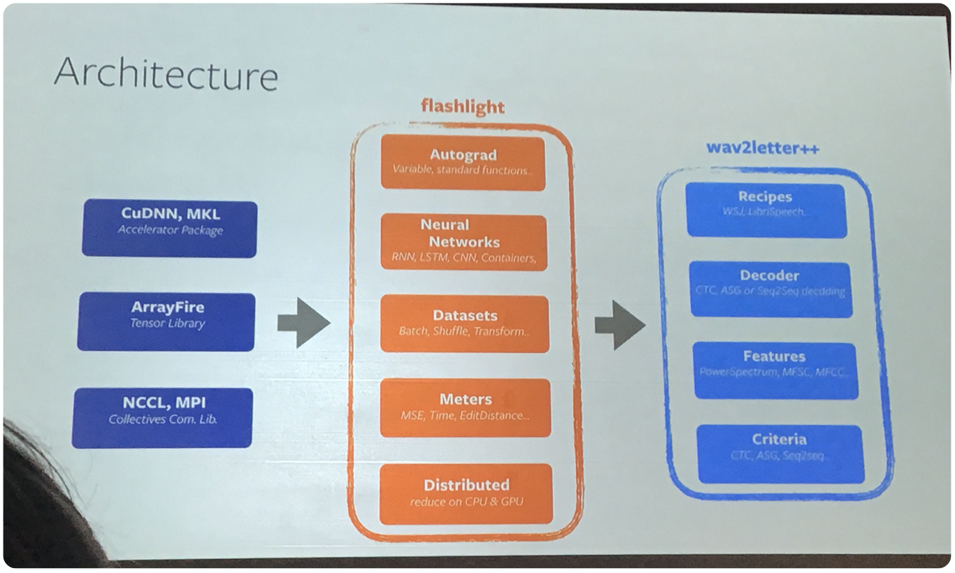
-
wav2letter++: Finally, Gabriel presented what is touted as the “fastest open-source speech recognition system”. The following is a diagram of the architecture:
4. Ron Weiss (Google)
Weiss’ talk was about progress in speech-to-speech generation at Google, and was mainly divided into 3 parts: (i) Speech-to-text translation, (ii) Parrotron, and (iii) Translatotron. The popular LAS model and Tacotron are used as building blocks for most of these tasks.
-
Speech-to-text translation: This is the task of transcribing an utterance in Language A into text in Language B. Traditionally, a cascading ASR+MT architecture has been used to tackle this problem. In their Interspeech’17 paper, they found that their end-to-end system was comparable to a cascading baseline, and multi-task learning improved the performance. MT was performed by co-training an auxiliary ASR system. In a follow-up paper, they scale up their system significantly (1300h of translated speech and 49k of transcribed speech) and found that although a cascading system is better, pretraining and MT eliminates the gap.
-
Parrotron: This is a system for voice conversion (many-to-ne conversion to Google’s generic voice). They use synthesized training data using a parallel WaveNet. A demo played during the talk was very well received.
-
Translatotron: This is a system for speech-to-speech translation. In their first attempt to get such a system to work using the simple ST pipeline, they found that the system just babbled (although with an auxiliary decoder, it was able to get short phrases and common words right). However, using someo of the lessons learnt from their other seq2seq systems (primarily the importance of multitask training), they were able to build a competitive system.
There were also some other interesting talks which I haven’t detailed here:
- Kristen Grauman (UT Austin/Facebook), on visually guided audio source separation.
- Simon Doclo (Univ. of Oldenburg), on noise reduction and dereverberation algorithms.
- Hirokazu Kameoka (NTT), on voice conversion using image-to-image translation (like CycleGANs) and seq2seq learning approaches.
Posters
The complete list of posters can be found here. Most of the presented work was in the domain of audio source separation/classification and signal processing in general, which is outside my domain of research. However, I found 2 very interesting posters that I spent most of my time at.
1. Using TTS to learn SLU
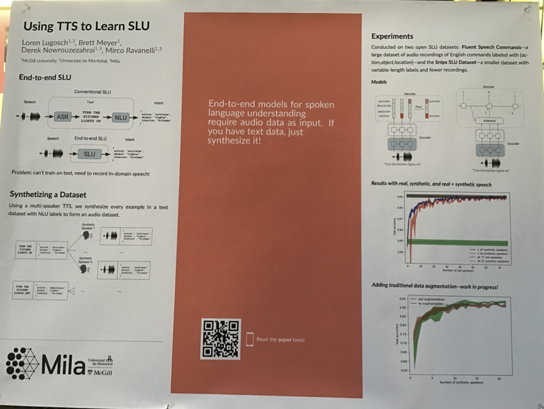
Key ideas:
- In-domain data for end-to-end SLU is limited - so use speech synthesis to generate training data.
- Each example in the training set is fed to 22 synthetic speakers, and this synthesized speech is used for training the system. The TTS system used is Facebook’s VoiceLoop.
- Test accuracy increases with number of synthetic speakers.
Although the idea is simple, there has been immense interest recently for using TTS systems for augmentation in ASR, especially since synthesis seems to have become better. It is not a new idea (backtranslation style augmentation, and one-hot speaker adaptation has been done earlier), but it is probably helping more now because of advances in TTS.
2. Self-normalizing deep CNNs with SELUs
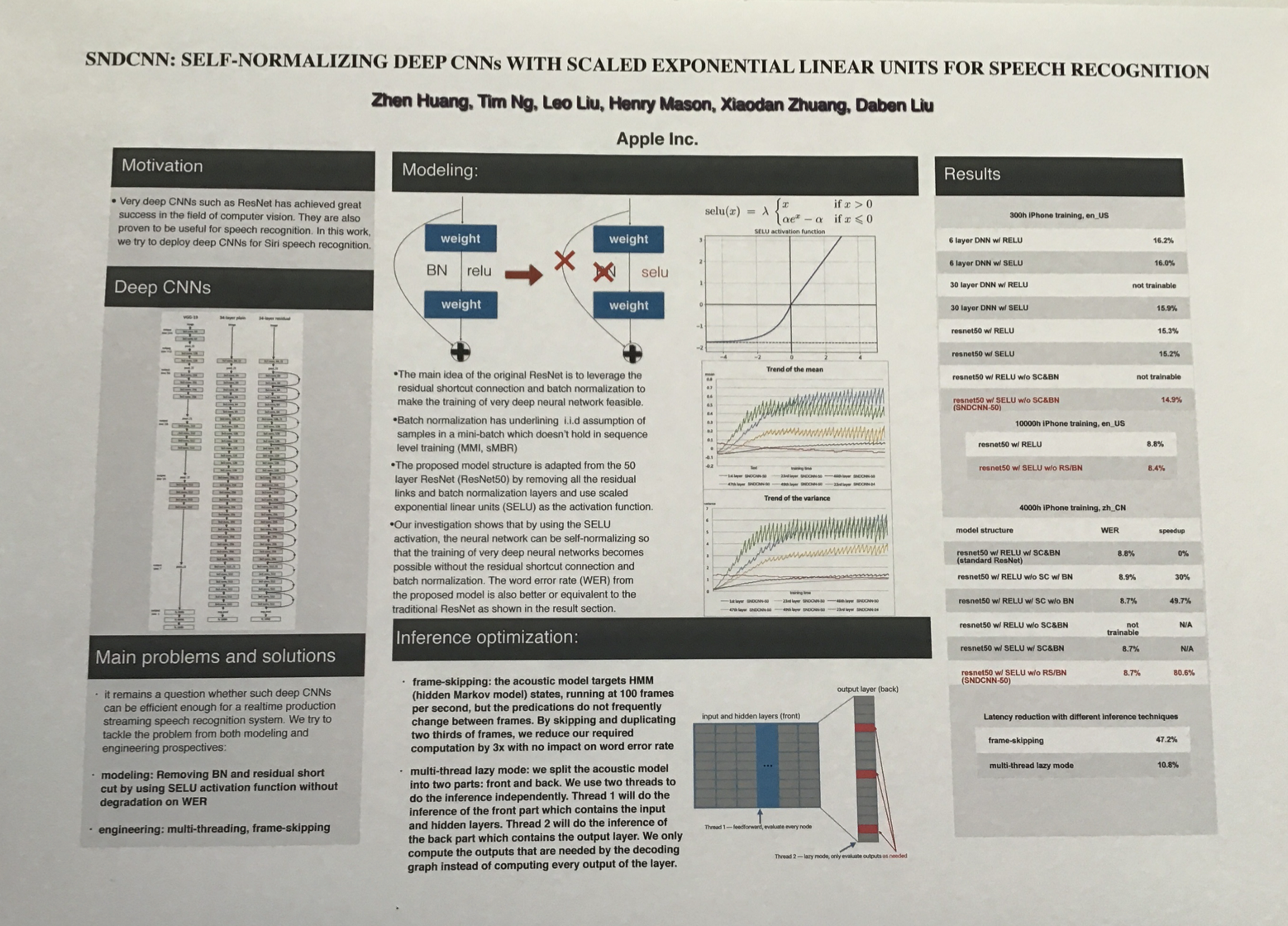
Key ideas:
- Deep convolutional models used in acoustic modeling often have residual connections and batch normalization.
- Removing these can make the model faster, but also worsen WER. Is there a way to remove these and keep the performance similar?
- Yes! Use scaled exponential linear unit (SELU) as the activation function. I found this post useful.
- Using SELU makes it possible to train very deep CNNs. Experiments with 300h and 4000h of (in-house) data showed consistent performanceon WER evaluation and up to 80% speedup during inference.