An Introduction to Speech Recognition using WFSTs

Until now, all of my blog posts have been about deep learning methods or their application to NLP. Since the last couple of weeks, however, I have started learning about Automatic Speech Recognition (ASR)¹.

The ASR logic is very simple (it’s just Bayes rule, like most other things in machine learning). Essentially, given a speech waveform, the objective is to transcribe it, i.e., identify a text which aligns with the waveform. Suppose $Y$ represents the feature vectors obtained from the waveform (Note: this “feature extraction” itself is an involved procedure, and I will describe it in detail in another post), and $\mathbf{w}$ denotes an arbitrary string of words. Then, we have the following.

The two likelihoods in the term are trained separately. The first component, known as acoustic modeling, is trained using a parallel corpus of utterances and speech waveforms. The second component, called language modeling, is trained in an unsupervised fashion from a large corpus of text.

Although the ASR training appears simple from this abstract level, the implementation is arguably more complex, and is usually done using Weighted Finite State Transducers (WFSTs). In this post, I’ll describe WFSTs, some of their basic algorithms, and give a brief introduction to how they are used for speech recognition.

Weighted Finite State Transducers (WFSTs)

If you have taken any Theory of Computation course before, you’d probably already be aware what an automata is. Essentially, a finite automaton accepts a language (which is a set of strings). They are represented by directed graphs as shown below.

Each such automaton has a start state, one or more final states, and labeled edges connecting the states. A string is accepted if it ends in a final state after traversing through some path in the graph. For instance in the above DFA (deterministic finite automata), a, ac, and ae are allowed.

So an acceptor maps any input string to a binary class {0,1} depending on whether or not the string is accepted. A transducer, on the other hand, has 2 labels on each edge — an input label, and an output label. Furthermore, a weighted finite state transducer has weights corresponding to each edge and every final state.

Therefore, a WFST is a mapping from a pair of strings to a weight sum. The pair is formed from the input/output labels along any path of the WFST. For pairs which are not possible in the graph, the corresponding weight is infinite.

In practice, there are libraries available in every language to implement WFSTs. For C++, OpenFST is a popular library, which is also used in the Kaldi speech recognition toolkit.

In principle, it is possible to implement speech recognition algorithms without using WFSTs. However, these data structures have several proven results² and algorithms which can directly be used in ASRs without having to worry about correctness and complexity. These advantages have made WFSTs almost omniscient in speech recognition. I’ll now summarize some algorithms on WFSTs.

Some basic algorithms on WFSTs

Composition

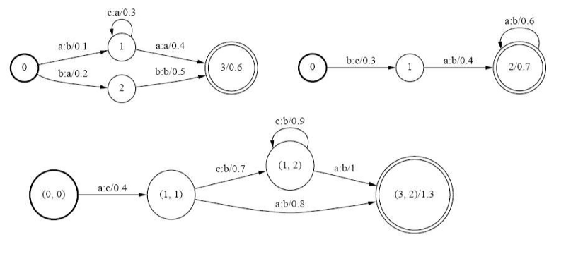
Composition, as the name suggests, refers to the process of combining 2 WFSTs to form a single WFST. If we have transducers for pronunciation and word-level grammar, such an algorithm would enable us to form a phone-to-word level system easily.

Composition is done using 3 rules:

1. Initial state in the new WFST are formed by combining the initial states of the old WFSTs into pairs.
2. Similarly, final states are combined into pairs.
3. For every pair of edges such that the o-label of the first WFST is the i-label of the second, we add an edge from the source pair to the destination pair. The edge weight is summed using the sum rules.

An example of composition is shown below.

At this point, it may be important to define what “sum” means for edge weights. Formally, the “languages” accepted by WFSTs are generalized through the notion of semirings. Basically, it is a set of elements with 2 operators, namely $\oplus$ and $\otimes$. Depending on the type of semiring, these operators can take on different definitions. For example, in a tropical semiring, $\oplus$ denotes $\min$, and $\otimes$ denotes sum. Furthermore, in any WFST, weights are $\otimes$-multiplied along paths (Note: here “multiplied” would mean summed for a tropical semiring) and $\oplus$-summed over paths with identical symbol sequence.

See here for OpenFST implementation of composition.

Determinization

A deterministic automaton is one in which there is only one transition for each label in every state. By such a formulation, a deterministic WFST removes all redundancy and greatly reduces the complexity of the underlying grammar. But, are all WFSTs determinizable?

The Twins Property: Let us consider an automaton A. Two states p and q in A are said to be siblings if both can be reached by string x and both have cycles with label y. Essentially, siblings are twins if the total weight for the paths until the states, as well as that including the cycle, are equal for both.

A WFST is determinizable if all its siblings are twins.

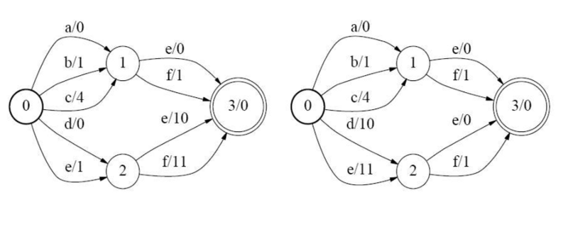
This is an example of what I said earlier regarding WFSTs being an efficient implementation of the algorithms used in ASR. There are several methods to determinize a WFST. One such algorithm is shown below.

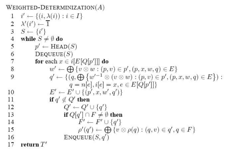
In simpler steps, this algorithm does the following:

• At each state, for every outgoing label, if there are multiple outgoing edges for that label, replace them with a single edge with weight as the $\otimes$-sum of all edge weights containing that label.

Since this is a local algorithm, it can be efficiently implemented in-memory. To see how to perform determinization in OpenFST, see here.

Minimization

Although minimization is not as essential as determinization, it is still a nice optimization technique. It refers to minimizing the number of states and transitions in a deterministic WFST.

Minimization is carried out in 2 steps:

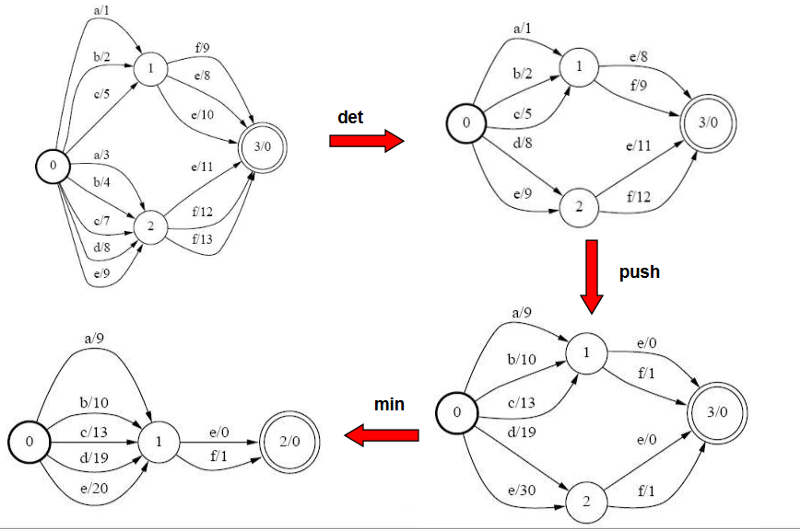
1. Weight pushing: All weights are pushed towards the start state. See the following example.

1. After this is done, we combine those states which have identical paths to any final state. For example in the above WFST, states 1 and 2 have become identical after weight pushing, so they are combined into one state.

In OpenFST, the implementation details for minimization can be found here.

The following³ shows the complete pipeline for a WFST reduction.

WFSTs in speech recognition

Several WFSTs are composed in sequence for use in speech recognition. These are:

1. Grammar (G): This is the language model trained on large text corpus.
2. Lexicon (L): This encodes information about the likelihood of phones without context.
3. Context-dependent phonetics (C ): This is similar to n-gram language modeling, except that it is for phones.
4. HMM structure (H): This is the model for the waveform.

In general, the composed transducer HoCoLoG represents the entire pipeline of speech recognition. Each of the components can individually be improved, so that the entire ASR system gets improved.

This was just a brief introduction to WFSTs which are an important component in ASR systems. In further posts on speech, I hope to discuss things such as feature extraction, popular GMM-HMM models, and latest deep learning advances. I am also reading papers mentioned here to get a good overview of how ASR has progressed over the years.