These are my notes from reading the Ultra-scale Playbook by HuggingFace. These are only meant for quick review and summary of concepts.
Introduction
There are 3 main components for large-scale training:
- Training needs to fit in memory.
- GPUs should not sit idle, i.e., compute efficiency is important.
- We should overlap communication overhead with compute.
The general flow of training is 3 steps:
- A forward pass to compute the outputs given the inputs.
- A backward pass to compute the gradients.
- An optimizer step to update the weights based on the gradients.
Batch size: One of the main requirements for training well is to have large enough batches. Modern LLMs are usually trained with batch size of 4–60 million tokens.
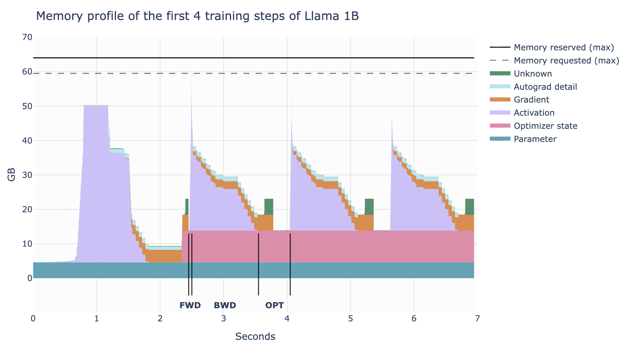
Memory usage in Transformers
The following need to be stored in memory:
- Model weights
- Model gradients
- Optimizer states
- Activations (needed to compute the gradients)
Of these, the first 3 depend on the model and floating-point precision, whereas the last depends on the input size.
Scaling up training is a question of maximizing compute efficiency while keeping the memory requirements of these various items within the memory constraints of the GPU.
- Number of params is quadratic in hidden dimension.
- For basic FP32 training, each floating point needs 4 bytes, so we need:
- 4 * N bytes for the model weights
- 4 * N bytes for the model gradients
- 8 * N bytes for the optimizer states, since Adam stores coeffs for 1st and 2nd order moments
Memory for activations
- Memory scales linearly with the batch size but quadratically with the sequence length.
- As a result, it takes up significant memory after 2-4k tokens.
- To avoid this, we can use activation recomputation (also called gradient checkpointing).
- In this method, instead of storing all the activations, we discard some of them and recompute them during the backward pass.
- Which activations to discard? Which have high storage cost but low recomputation cost — attention layer activation!
- FlashAttention already uses activation recomputation in its optimization strategy.
- To deal with growing memory with batch size, we can use gradient accumulation: process smaller micro-batches (forward + backward), accumulate gradients from all, and then run the optimizer step.
Communication primitives
Before getting into the parallelism, let us summarize the major communication primitives.
| Primitive | What it does? |
|---|---|
| Broadcast | Share some data from one node to all other nodes. |
| Reduce | Aggregate data from all nodes through some function. |
| AllReduce | Reduce followed by broadcast to all nodes. |
| Gather | Collect chunks of data from all node into one node. |
| AllGather | Gather followed by broadcast to all nodes. |
| Scatter | Scatter chunks of data from one node to all nodes. |
| ReduceScatter | Aggregate data from all nodes through some function, and scatter chunks of the output to all nodes. |
- In practice, AllReduce is often implemented as ReduceScatter + AllGather.
Data parallelism
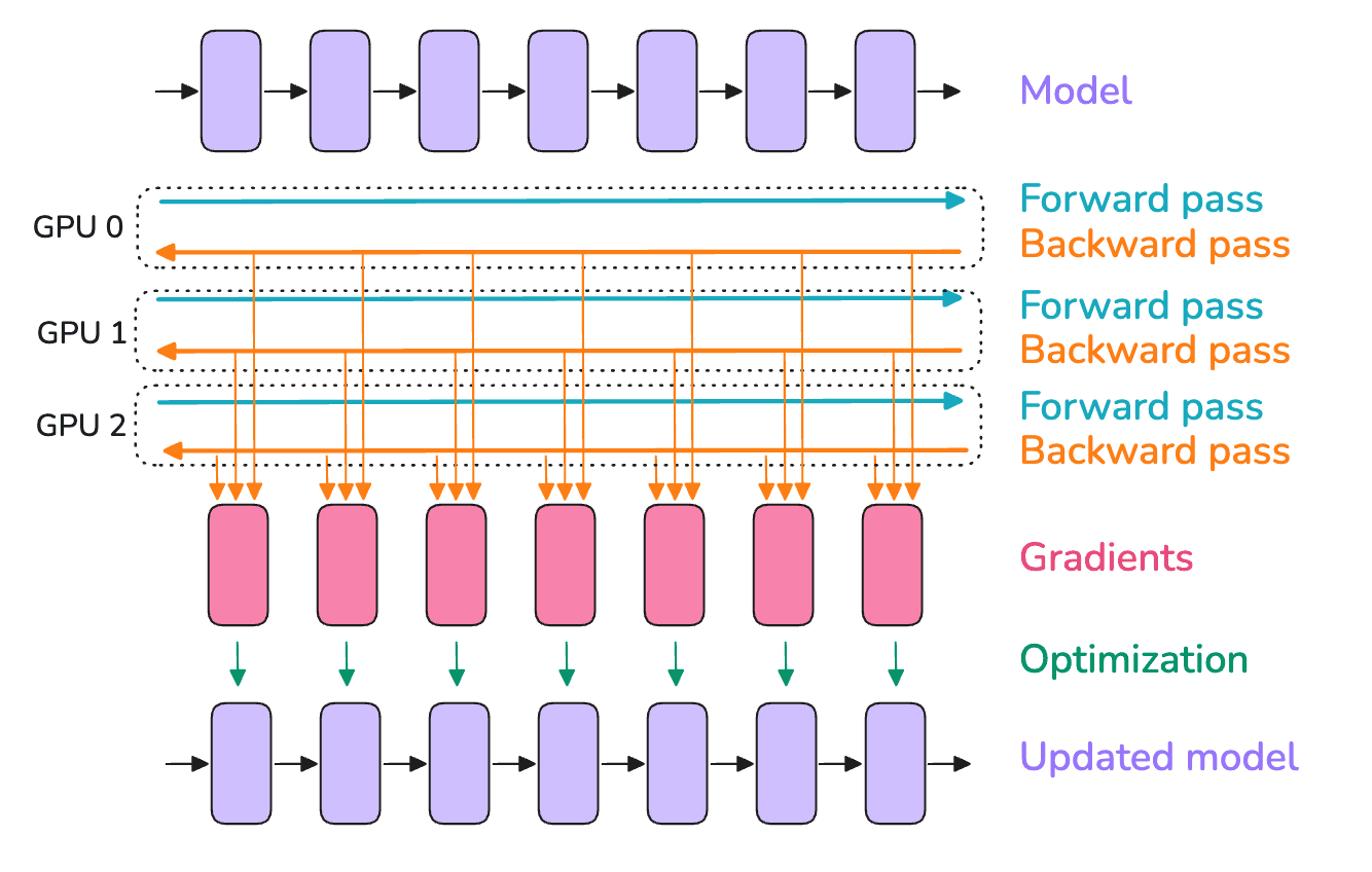
- In DP, we run forward and backward on micro-batches on different GPUs.
- The gradients are then averaged across all GPUs using AllReduce.
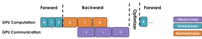
- In a naive implementation, the AllReduce will happen after backward is complete for all layers, but we want to overlap computation with communication as much as possible.
Optimizations to improve DP
- Overlap gradient synchronization with backward pass by attaching an all-reduce hook to each parameter.
- Run the all-reduce in buckets (e.g. per layer) instead of per parameter to reduce communication overhead.
- If using gradient accumulation, only run all-reduce after gradient from all micro-batches are accumulated in each GPU.
Limitations of DP
- As # GPUs increases, the overhead of synchronizing the gradients becomes too much, which affects the training throughput.
- It assumes that the model can fit on a single GPU.
So what else can we do when the model is too big?
- Sharding (DeepSpeed ZeRO or PyTorch FSDP)
- Parallelism (tensor, context, pipeline)
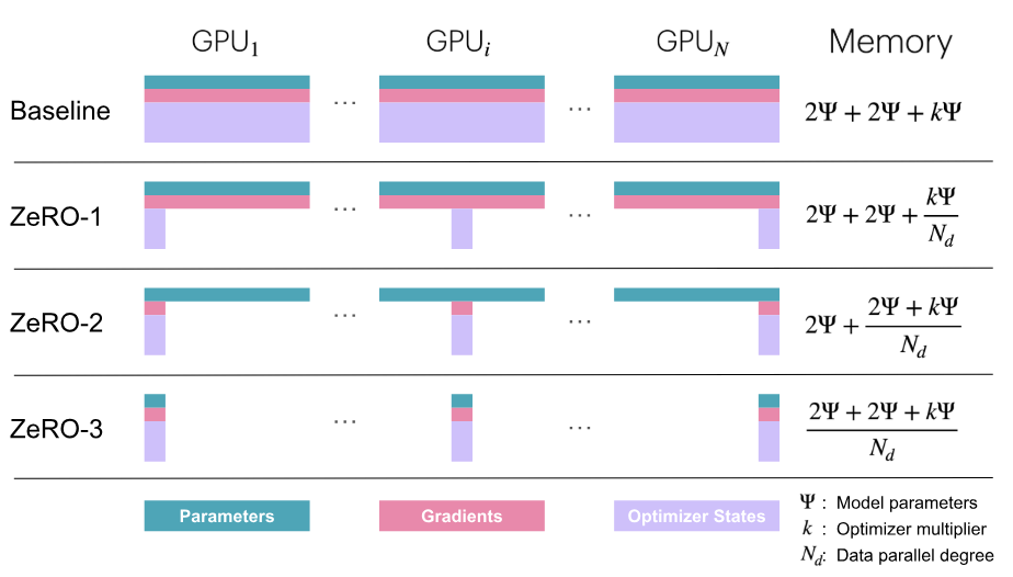
Sharding (Zero Redundancy Optimizer)
- There is a lot of redundancy in DP because the model weights, gradients, and optimizer states have to be copied on each GPU.
- ZeRO partitions these across ranks:
- ZeRO-1: optimizer state
- ZeRO-2: optimizer state + gradient
- ZeRO-3: optimizer state + gradient + weights; also called fully-sharded DP (FSDP)
ZeRO-1
- In vanilla DP, all ranks gather the gradients and perform identical optimizer steps. This is a lot of wasted effort.
- How it works:
- Each rank does forward pass on full weights.
- Each rank does backward pass on full weights.
- ReduceScatter on the gradients.
- Each rank performs the optimizer step on its subset of optimizer states.
- AllGather to share updated weights to all ranks.
ZeRO-2
- If optimizer is only updating a subset of the weights, we don’t need all the gradients on each rank.
- In ZeRO-2, each rank only stores a subset of gradients.
- During backward pass, instead of performing AllReduce on gradients, we only need ReduceScatter.
ZeRO-3
- Also shard the model weights. But then, how will we do forward and backward passes?
- As we go through the layers, AllGather the weights, and immediately flush them after computation.
- During backward, AllGather the weights again and ReduceScatter the computed gradients.
- This requires a lot of communication overhead, but we can overlap communication for next layer with computation for current layer. This is called prefetching.
Limitations of ZeRO
- It only works if a single layer can fit into memory.
- It cannot partition the activations (which scales quadratically with sequence length).
Tensor Parallelism
- It can shard weights, gradients, optimizer states, and activations without any communication between GPUs!
- It is based on simple properties of matmul.
- Suppose we want to do $X \cdot W$, where $X$ is the input ($BT \times D$) and $W$ is the weight matrix ($D \times d_{\text{emb}}$).
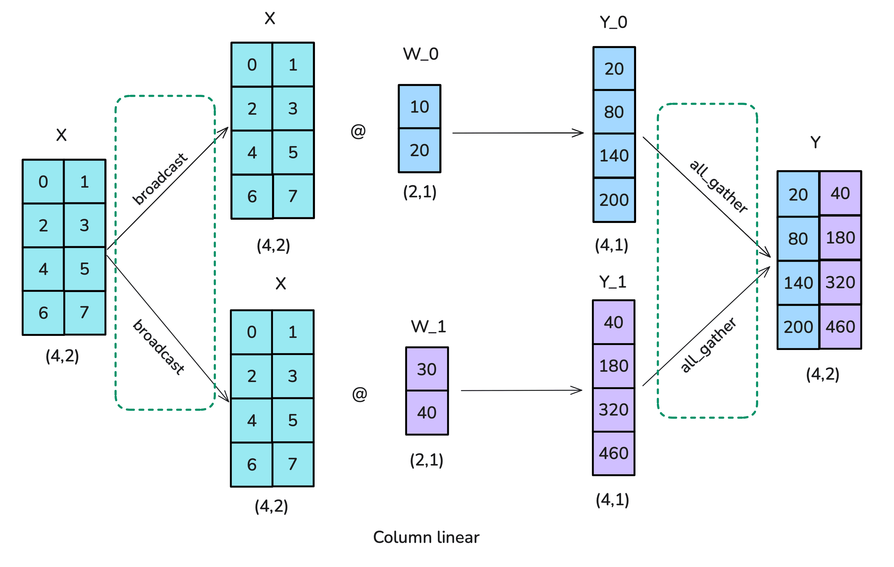
Column-linear
- Split $W$ into columns and send one column to each rank.
- Broadcast $X$ to all ranks, and run matmul on each rank.
- AllGather the outputs to create the result matrix.
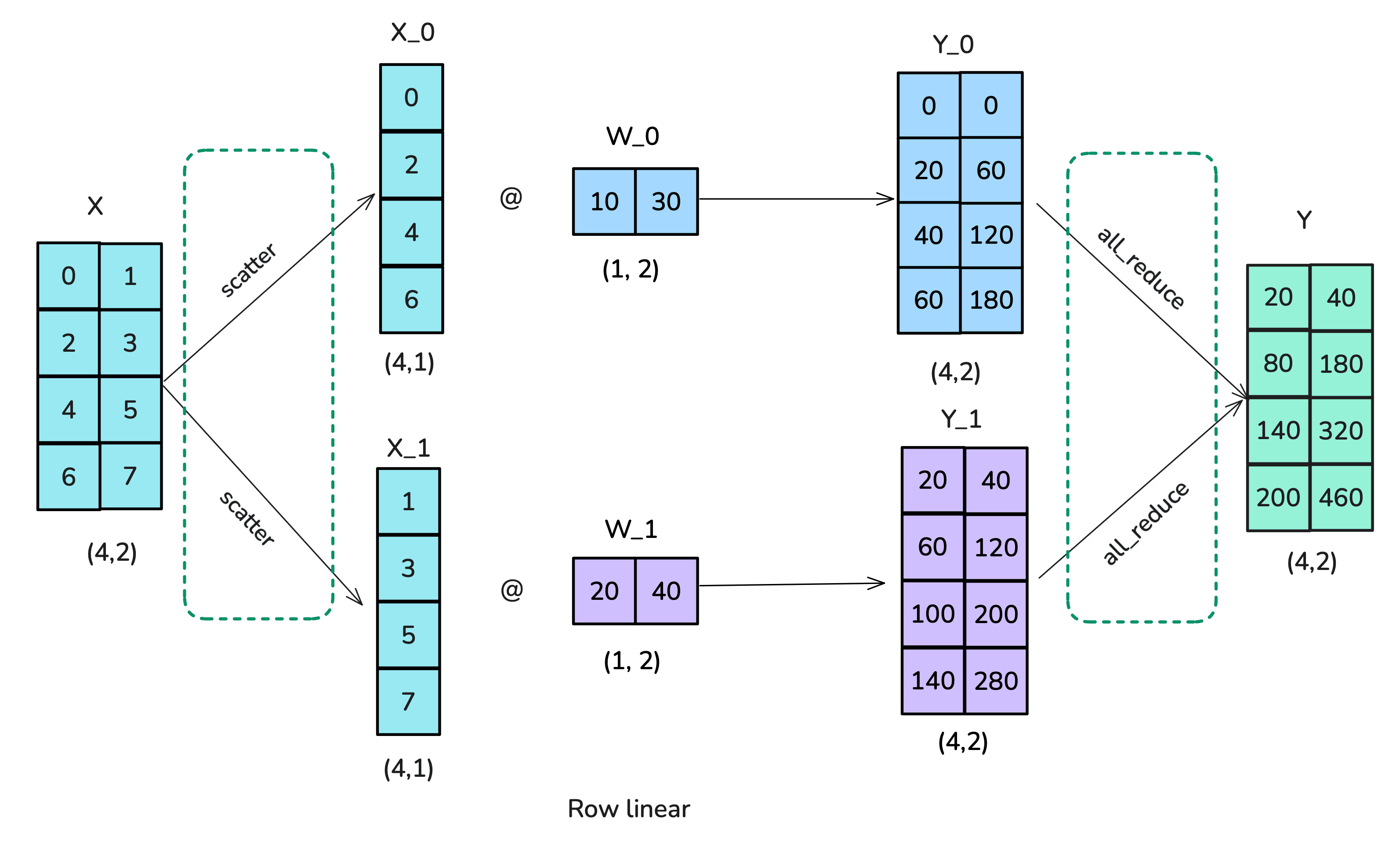
Row-linear
- Split $W$ into rows and send one row to each rank.
- Scatter $X$ columns across ranks (so that matmul is valid).
- Run matmul on each rank.
- AllReduce the outputs to create the result matrix.
TP in a transformer block
- A transformer block contains 2 components:
- Multi-layer perceptron (MLP) with 2 feedforward layers
- Multi-head attention (MHA)
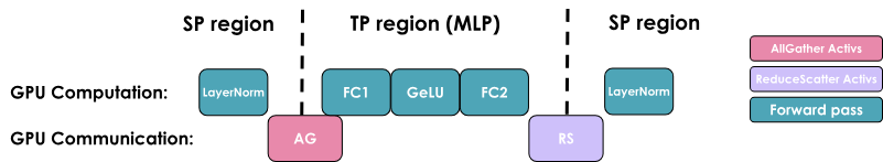
- For the MLP component:
- Use column linear on the first FFN and row-linear on the second.
- This means we need to Broadcast the inputs in the beginning, and AllReduce at the end.
- Parallelism is applied along the hidden dimension.
- For the MHA component:
- Split the $Q$, $K$, $V$ matrices in column-linear way across ranks.
- Broadcast $X$ and do self-attention on each rank.
- AllReduce on the outputs before dropout.
- Unlike MLP, we apply parallelism along the heads dimension, so we need to make sure that TP degree <= number of heads.
Limitations of TP
- We still need to run AllReduce before layer norm, which adds communication overhead.
- Usually we keep TP to only within a single node to utilize fast NVLink interconnects.
- Operations like dropout and layer-norm still require the full hidden dimension.
Unlike data-parallel, since TP partitions matrices across ranks, it is non-trivial to compute the gradients on each rank. See this blog for derivation.
Sequence parallelism
- Since TP cannot work for layer-norm and dropout, we instead use sequence parallelism.
- This means partitioning the input along the sequence dimension for these operations.
- Similar to vanilla TP, TP + SP is only done within a node (i.e., rank <= 8).
Context parallelism
- When processing very long sequences (like 128k), we can still go out of memory in the TP region (i.e., MLP and MHA).
- Context parallelism is same as sequence parallelism, but it is applied on the TP modules.
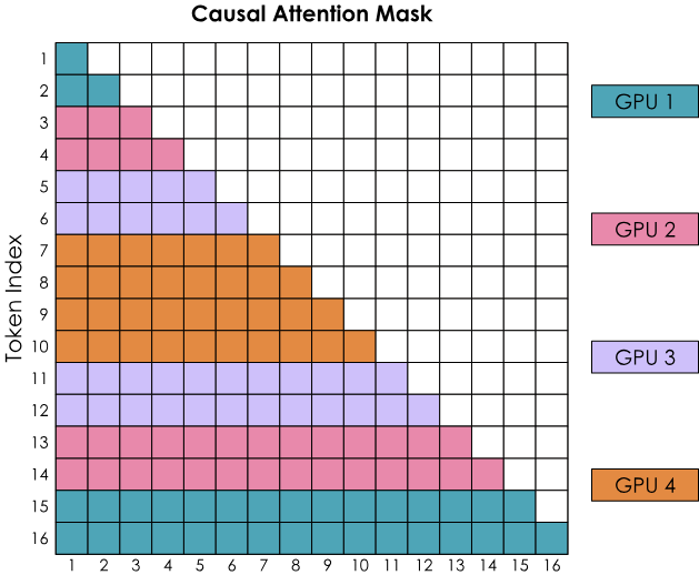
- But how will self-attention work now if the sequence is split across ranks? The answer is ring attention.
- Suppose there are $K$ ranks, and the sequence is split across them. The attention computation will be completed in $K$ steps.
- In each step, the rank sends its current key-values to the next rank (in a ring), while at the same time performing computation on the key-values it has.
- But causal attention mask will lead to an imbalance in compute across ranks! We can solve this using zig-zag ring attention:
- Instead of splitting the sequence uniformly, ensure that each rank has a mix of early and late tokens.
Pipeline parallelism
- TP only works well within a single node (i.e. at most 8 ranks). Beyond that, the communication overhead is too much due to slower network bandwidth.
- SP and CP can help with long sequences, but what if the size of the model itself is too big to fit on 8 GPUs? This is the case for models larger than ~70B.
- Answer: split the model layers across nodes, e.g., layers 1–4 on rank 1, layers 5–8 on rank 2, and so on. This is called pipeline parallelism.
- PP reduces memory due to weights, gradients, and optimizer states, but there are no savings in activation memory. Why?
- This is because each GPU still needs to do all the forward passes before starting the backward pass.
- The main challenge in PP is: how to effectively keep all GPUs busy at all times?
- The GPU idle time is known as bubble. Our goal is to reduce this bubble as much as possible!
Naive PP
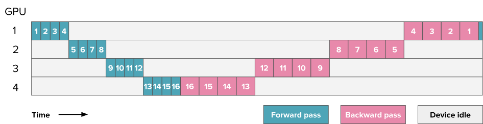
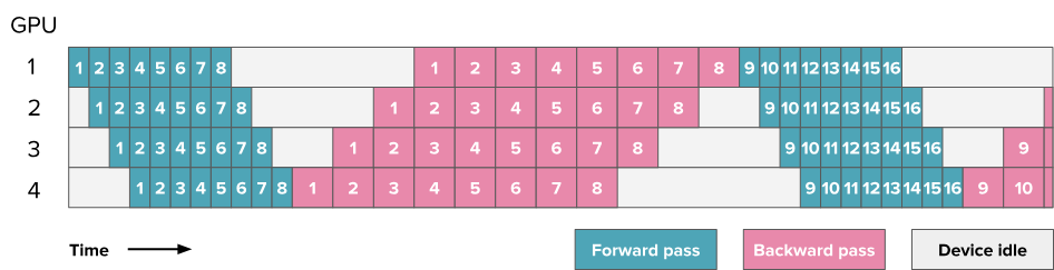
AFAB schedule
- Split each batch into micro-batches which can be almost processed in parallel.
Expert parallelism
- Since the feedforward layers are independent, we can split them across ranks.
- EP is usually used along with DP and TP, since it does not split the data or the self-attention.
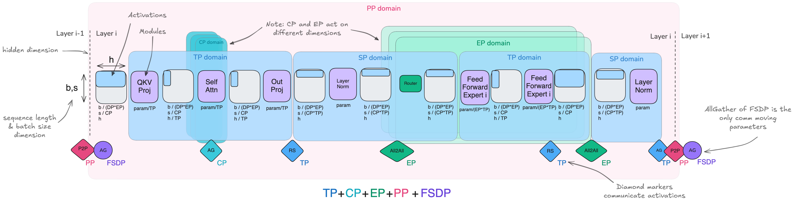
Summary of 5D parallelism
- DP = along the batch dimension
- TP = along the hidden dimension
- SP/CP = along the sequence dimension
- PP = along the model layers
- EP = along the FFN experts
DP also includes ZeRO strategies to shard optimizer states, gradients, and parameters.
Combination of methods
- ZeRO-3 and PP both solve weight partitioning but in different ways, so they are usually not combined.
- But PP can be combined easily with ZeRO-1 or ZeRO-2 (done in DeepSeek-v3).
- TP + SP can also be combined with the above setting. TP is kept for high-speed communication while PP can tolerate low-speed.
Finding the best training configuration
- First we need to fit the model on our GPUs:
- For small models (< 10B), use either TP or Zero-3 with full recompute on 8 GPUs.
- For medium models (10-100B), use one of: (i) TP=8 with PP, (ii) TP=8 with ZeRO-3.
- If you have a lot of GPUs (512+), definitely use TP=8 and optionally add PP.
- Special considerations: use CP for long context, and EP for MoE models.
- Next, we need the right global batch size. This is done by setting DP ranks or grad accumulation appropriately.
- Finally, we want to optimize train throughput:
- Scale up TP –> should ideally be equal to node size.
- Increase DP until it becomes a bottleneck, then add PP.
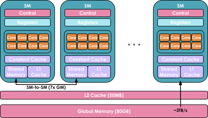
Deep dive into GPUs
- GPUs are organized into: compute and memory.
- On the compute side, an H100 GPU contains 132 SMs (streaming multiprocessors) with 128 cores per SM.
- On the memory side, the levels are: (i) registers (private to a thread), (ii) shared memory and L1 cache (shared between threads running on a single SM), (iii) L2 cache (shared between all SMs), and (iv) global memory (e.g. 80GB for H100).
- A kernel is a piece of code that runs on a single core. It can be written in CUDA or Triton.
- A host code prepares the data and code for each core.
- Threads are grouped into warps (32 threads per warp), which are further grouped into blocks (e.g., 512/1024 threads per block).
- An SM can run several blocks in parallel.
How to write a kernel?
- First option would be to use
@torch.compiledecorator and start with the generated Triton code (print usingexport TORCH_LOGS="output_code") - But Triton is limited to scheduling blocks across SMs. For more control, use CUDA.
- CUDA kernels are often used for the following frequent cases:
- Memory coalescing –> ensure that threads in a warp access consecutive memory locations
- Tiling –> instead of each thread loading rows from A and B, load a block into shared memory just once and let all threads reuse the shared data.
- Thread coarsening –> merge multiple threads to prevent I/O bottleneck in reading from shared memory
- Minimizing control divergence –> threads within the same block should not have different control paths, i.e., if-else.
Fused kernels
- We want to avoid going back and forth between host and GPU kernel commands.
- To do this, we pack as many successive computations as possible together into a single kernel, called a “fused kernel”.
- This is easy to do when there are consecutive point-wise operations, such as FFN + LayerNorm.