A few days ago, I conducted a poll soliciting opinions about the following question:
For the same parameter size, network architecture, and training data, which of the following models do you think would perform best at streaming ASR?
For the same parameter size, network architecture, and training data, which of the following models do you think would perform best at streaming ASR?
— Desh Raj (@rdesh26) October 26, 2025
It seems like a simple enough question, but I found the opinions rather conflicting. For the same model size, a transducer should rightly outperform a CTC model, as pointed out by the majority of people. But why did AED models not get any takers? And what about decoder-only models, which are a relatively new entry to this field?
In this post, let us try to answer this question from first principles!
Problem setup
Let us start with the following setup: we have an audio represented by a sequence of acoustic features $\mathbf{X} = (\mathbf{x}_1, \mathbf{x}_2, \ldots, \mathbf{x}_T)$, where $T$ is the length of the sequence and $\mathbf{x}_t \in \mathbb{R}^D$ is the $D$-dimensional feature vector at time $t$. These are usually log Mel-filterbank features, with $D=80$. Then, ASR can be formulated as a maximum a-posteriori (MAP) estimation problem:
\[\begin{align} \hat{\mathbf{y}} &= \arg\max_{\mathbf{y}} P(\mathbf{y} \mid \mathbf{X}) \\ &= \arg\max_{\mathbf{y}} \prod_{u \in U} P(y_u \mid \mathbf{y}_{<u}, \mathbf{X}) \end{align}\]Here, $y_u \in \mathcal{Y}$ are the output units, such as characters, phonemes, or BPE units. Since the true distribution $P$ is unknown, we usually resort to a parameterized model $P_{\Theta}$ to approximate it. The parameters $\Theta$ are usually learned by maximizing the log-likelihood of the training data:
\[\Theta^* = \arg\max_{\Theta} \mathbb{E}_{(\mathbf{X},\mathbf{y})\sim \mathcal{D}} \log P(\mathbf{y} \mid \mathbf{X}; \Theta).\]After the model (i.e., $\Theta$) is trained, we can use it to estimate the most likely output sequence $\hat{\mathbf{y}}$ for a given input sequence $\mathbf{X}$ using the MAP estimation rule above. Since it is intractable to compute the exact MAP estimate, we usually resort to approximate algorithms such as beam search or Viterbi decoding.
Frame-synchronous v/s label-synchronous
Before we get into the details of the different models, let us first distinguish between two types of models: frame-synchronous and label-synchronous.
- A frame-synchronous model is driven by the input, i.e., it takes one frame of the input at each time-step and makes a prediction, stopping after the last input frame is processed. At any step in decoding, the model is aware of what frame index it is currently at, making it a natural choice for streaming tasks.
- A label-synchronous model is driven by the output, i.e., it predicts the output label-by-label, usually relying on the entire input as context.
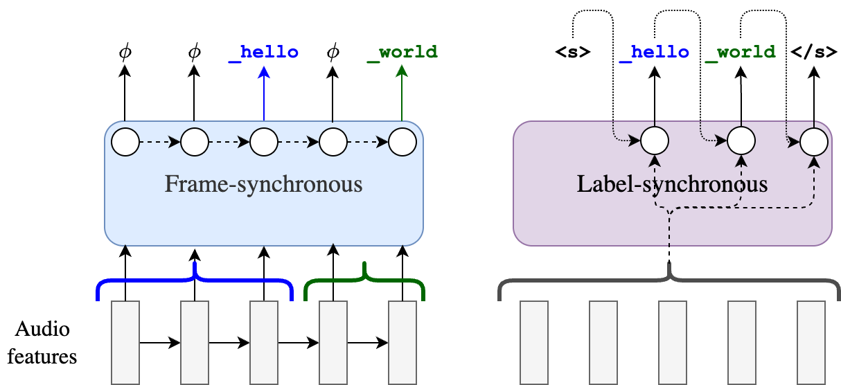
- CTC and RNN-T are examples of frame-synchronous models, as we will see in a bit.
- AED models (like Whisper) are label-synchronous.
Can you guess whether decoder-only models are frame-synchronous or label-synchronous?
The synchronicity difference between the different ASR models is purely based on inference method. All models are still trained using maximum likelihood estimate, i.e., by minimizing the negative log-likelihood $-\log P(\mathbf{y}\mid \mathbf{X})$. The main source of difference lies in how this probability distribution is approximated. In the next section, we will look at each model in detail to understand how it estimates $P(\mathbf{y}\mid \mathbf{X})$.
How do models estimate $P(\mathbf{y}\mid \mathbf{X})$?
CTC
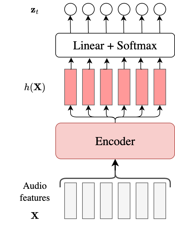
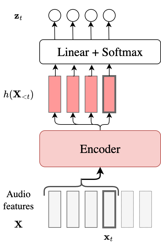
- The audio $\mathbf{X}$ is passed to an encoder to generate hidden representations $h(\mathbf{X})$.
- A simple linear layer followed by softmax generates probabilities over the vocabulary $\mathcal{Y} \cup {\phi}$, where $\phi$ is the CTC blank label. Here, the model makes an assumption that given $\mathbf{X}$, the output label at any step is conditionally independent of all earlier labels.
Instead of using the vanilla beam search, we modify it such that the beam always contains the top-$K$ final sequences $\mathbf{y}$ at any time-step (instead of the top-$K$ alignments $\mathbf{a}$). For more details about CTC beam search, please refer to this excellent article.
Anyway, for the purpose of our analysis, it suffices to note the following:
- Conditioning on $\mathbf{X}$ is approximated through $h_t(\mathbf{X})$, so the assumption is that the encoder is strong enough to capture all relevant information in $\mathbf{X}$.
- There is no conditioning on $\mathbf{y}_{<u}$, which is quite a strong assumption.
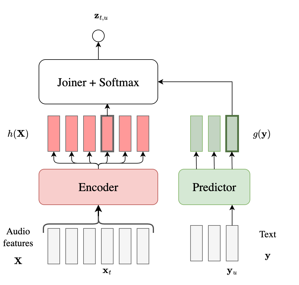
RNN-T
RNN-T relaxes this conditional independence assumption by additionally conditioning the output on the previous tokens as shown below. In addition to the audio encoder, it adds a predictor and a joiner. The predictor autoregressively models the output sequence, embedding it into high-dimensional representations $g(\mathbf{y})$. Note that these are only based on the text sequence, without any dependency on the audio. The joiner is usually just a linear layer which computes the logits at frame index $t$ and label index $u$.
We can again write out the probability estimate of the MAP posterior as follows:
\[\begin{align} P(\mathbf{y} \mid \mathbf{X}) &= \sum_{\mathbf{a}\in \mathcal{B}_{\mathrm{rnnt}}^{-1}(\mathbf{y})}P(\mathbf{a}\mid \mathbf{X}) \\ &= \sum_{\mathbf{a}\in \mathcal{B}_{\mathrm{rnnt}}^{-1}(\mathbf{y})} \prod_{t=1}^T P(a_t \mid \mathbf{a}_{<t},\mathbf{X}) \\ &= \sum_{\mathbf{a}\in \mathcal{B}_{\mathrm{rnnt}}^{-1}(\mathbf{y})} \prod_{t=1}^T \mathbf{z}_{t,u} \\ \end{align}\]We note the following:
- The conditioning on $\mathbf{X}$ is approximated similar to CTC.
- Unlike CTC, it does not ignore the output label dependency since $\mathbf{z}\_{t,u}$ is derived from both $h(\mathbf{X})$ and $g(\mathbf{y}_{<u})$.
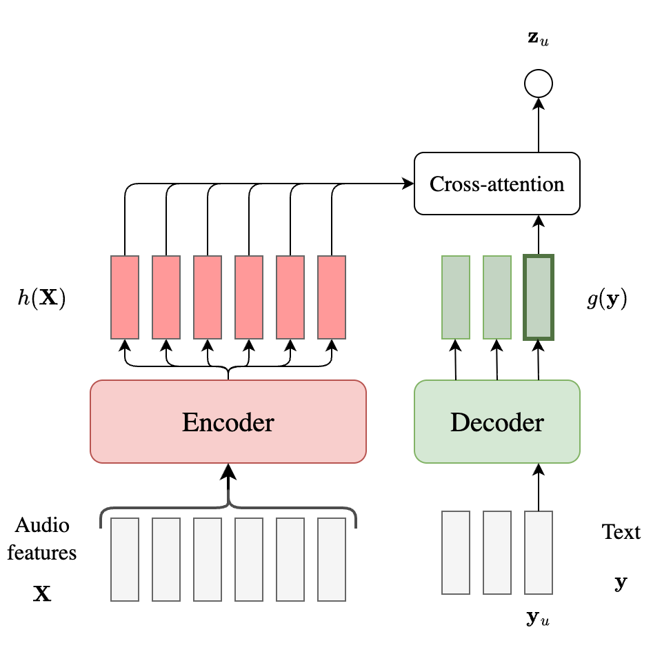
AED
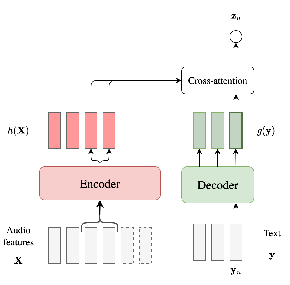
Attention-based encoder-decoder models also have an audio encoder $h(\mathbf{X})$ and a decoder $g(\mathbf{y})$ (analogous to the predictor in RNN-T). However, they use cross-attention to compute $\mathbf{z}_u$ which directly conditions on the full $h(\mathbf{X})$ instead of just the embedding at time $t$, as shown below.
Since AED models are label-synchronous, the probability factorization becomes simpler, since there is no need for marginalizing over alignments.
\[P(\mathbf{y} \mid \mathbf{X}) = \prod_{u=1}^U P(y_u \mid \mathbf{y}_{<u}, \mathbf{X}) = \prod_{u=1}^U \mathbf{z}_u\]In the context of our analysis, the note-worthy points are:
- AED models condition each output label on the entire audio $\mathbf{X}$ through cross-attention.
- The conditioning on $\mathbf{y}_{<u}$ is through the decoder state, similar to RNN-T.
Decoder-only
In the context of speech, the term ``decoder-only’’ is a slight misnomer, since most such papers still use a relatively strong audio encoder, often to convert the audio into discrete tokens. This is because the model has (unfortunately) become conflated with the popular LLM use case. For our analysis, however, we will still assume the original setup with the audio features $\mathbf{X}$. It is easy to see that we can map both text and audio into the same space for feeding into the decoder $g$ (shown below), through some simple linear transformation.
A decoder-only model can be used for non-streaming ASR by first prefilling the audio features (i.e., to update the KV cache in a single step), and then prompting the model with $\texttt{<s>}$ to start generating the corresponding transcript. This is shown below.
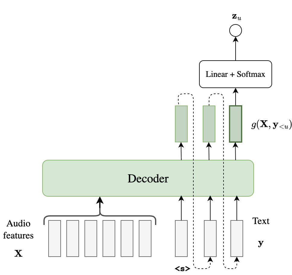
- Similar to AED, decoder-only models condition each output label on the entire audio $\mathbf{X}$, but they use layer-wise self-attention instead of cross attention.
- Unlike AED, the output conditioning is also through self-attention on all the previous $\mathbf{y}_{<u}$.
So who wins for non-streaming ASR?
Let us quickly recap the above discussion in a table.
| Model | Audio conditioning | Output conditioning |
|---|---|---|
| CTC | $h_t(\mathbf{X})$ only | None |
| RNN-T | $h_t(\mathbf{X})$ only | Through predictor state $g(\mathbf{y}_{<u})$ |
| AED | Cross-attention over full $h({\mathbf{X}})$ | Through decoder state $g(\mathbf{y}_{<u})$ |
| Decoder-only | Self-attention over $\mathbf{X}$ | Self-attention over all $\mathbf{y}_{<u}$ |
Evidently, the representational capacity of the models for learning complex distributions should be in the order: CTC < RNNT < AED < Decoder-only. However, the theoretical order may not be borne out in practice. For example:
- If the target distribution is fairly simple (e.g., voice commands), CTC would be sufficient. In practice, a CTC model combined with an external LM through shallow fusion (or rescoring) often provides a relatively strong baseline for ASR.
- Models with larger capacity will overfit quickly if not trained with enough data. This is the classic bias/variance trade-off from Machine Learning 101.
- The actual performance also depends on the architecture of the encoder/decoder networks. AEDs used to be the modeling choice for speech translation (where the speech-text alignment is not monotonic), but with the advent of strong Transformer-based encoders, RNN-Ts have also been shown to be adept at the task. For the ASR task which only requires monotonic alignment, the performance difference would be even less marginal.
Information-Theoretic View
From an information theory perspective, we can formalize the differences between these models in terms of mutual information $I(\mathbf{y}; \mathbf{X})$.
The optimal ASR model would maximize: \(I(\mathbf{y}; \mathbf{X}) = H(\mathbf{y}) - H(\mathbf{y} \mid \mathbf{X})\)
Each model makes architectural choices that effectively constrain this mutual information:
- CTC: Assumes $I(a_t; a_{<t} \mid \mathbf{X}) = 0$, losing label dependency information
- RNN-T: Captures $I(y_u; y_{<u} \mid \mathbf{X})$ but limits audio context to $h_t(\mathbf{X}_{\leq t})$
- AED: Full access to $I(y_u; \mathbf{X} \mid y_{<u})$ through cross-attention
- Decoder-only: Maximum modeling capacity for $I(\mathbf{y}; \mathbf{X})$
The case of streaming ASR
With this in mind, let us now turn our attention to streaming ASR, which was the entire point of my poll.
Thus far, we assumed that the model is allowed to condition on the entire audio sequence $\mathbf{X}$. In streaming ASR, this assumption does not hold, i.e., at any time-step, the model must make a decision based on the partial audio $\mathbf{X}_{<t}$.
From the perspective of the encoder $h$, the change is straightforward (at least in theory). Since most modern encoders are Transformer-based, the model can be made “causal” by modifying the attention mask to attend only to the left context. In practice, most implementations also allow for a few frames of right-context in the attention mask in what is known as a lookahead. This is known to improve WERs at the cost of a small increase in latency. With this change, we can now obtain encoder representations $h_t(\mathbf{X}_{<t})$ at any time-step $t$.
For frame-synchronous models (CTC and RNN-T), this encoder change is sufficient to convert the non-streaming model into a streaming one since their audio depend is only based on $h_t$. For this reason, these models are often called “naturally streaming”. Of course, the $h_t$ now does not contain information from the future, but that is an implication of the streaming task. If we take CTC as an example, here is how the processing flow changes:
Our MAP estimate now is not a true factorization, but an approximate. For example, here’s how it works out for the CTC model:
\[\begin{align} P(\mathbf{y} \mid \mathbf{X}) &= \sum_{\mathbf{a}\in \mathcal{B}^{-1}(\mathbf{y})}P(\mathbf{a}\mid \mathbf{X}) \\ &= \sum_{\mathbf{a}\in \mathcal{B}^{-1}(\mathbf{y})} \prod_{t=1}^T P(a_t \mid \mathbf{a}_{<t},\mathbf{X}) \\ &= \sum_{\mathbf{a}\in \mathcal{B}^{-1}(\mathbf{y})} \prod_{t=1}^T P(a_t \mid \mathbf{X}) \\ & \approx \sum_{\mathbf{a}\in \mathcal{B}^{-1}(\mathbf{y})} \prod_{t=1}^T P(a_t \mid \mathbf{X}_{<t}) \\ &= \sum_{\mathbf{a}\in \mathcal{B}^{-1}(\mathbf{y})} \prod_{t=1}^T z_t \\ \end{align}\]For label-synchronous models like AED, streaming ASR is more challenging. Without any concept of time alignment, how should the model know when to emit an output label? The standard answer to this is to replace the full cross-attention with a monotonic chunk-wise attention (MoChA). MoChA consists of two components:
- Monotonic attention: A hard attention mechanism that decides when to move to the next chunk of audio frames
- Chunk-wise attention: Soft attention within the selected chunk to compute the context vector
The chunk size becomes a hyperparameter that controls the latency-accuracy tradeoff: smaller chunks reduce latency but may hurt accuracy, while larger chunks improve accuracy at the cost of increased latency. Here’s a pictorial description of a streaming AED model.
Unlike CTC and RNN-T which can be trained by marginalizing on soft alignments (obtained through the backward probabilities), it is considerably more challenging to train streaming AED models, precisely due to the lack of alignments, but I will skip those details here.
The streaming constraint fundamentally alters the information available to each model. In non-streaming ASR, we had access to $I(\mathbf{y}; \mathbf{X})$, but in streaming, we can only access $I(\mathbf{y}; \mathbf{X}_{\leq t})$ at time $t$. This loss affects different models differently:
- CTC/RNN-T: The primary loss is $I(y_u; \mathbf{X}_{>t})$ from the encoder's limited context, but the decoding structure remains unchanged.
- AED with MoChA: Additional loss from chunked attention. Not only is $I(y_u; \mathbf{X}_{>t})$ unavailable, but the hard monotonic attention mechanism introduces approximation errors in $I(y_u; \mathbf{X}_{\leq t} \mid y_{<u})$ compared to full cross-attention.
In practice, this information-theoretic analysis suggests why frame-synchronous models (CTC/RNN-T) tend to be preferred for streaming ASR: they incur the smallest architectural penalty when transitioning from non-streaming to streaming modes. They are also no more difficult to train than their non-streaming versions. These arguments suggest why AED got precisely 0 votes in my poll: they are quite challenging to train well for streaming ASR, and do not offer any extra capacity over transducers.
So what about decoder-only models?
And now we finally come to decoder-only models for streaming ASR. Similar to AED, these models don’t have an internal concept of soft alignments, and so they must be trained with explicit hard alignments. This is usually done by interleaving the speech frames and text tokens based on forced alignments (with some delay). By leveraging self-attention over the entire prefix, the model should be able to condition on the full history of audio and text during decoding. This means that richer interactions can be modeled at the cost of more complex training.
A similar approach is through chunking, as proposed in the SpeechLLM-XL paper. Suppose we cut the input audio into fixed-sized chunks $(\mathbf{X}_1,\ldots,\mathbf{X}_K)$ and also split the corresponding transcript (based on alignments) into segments, with $\tilde{\mathbf{y}} = (\tilde{\mathbf{y}}_1,\ldots,\tilde{\mathbf{y}}_k,\ldots,\tilde{\mathbf{y}}_K) = (\mathbf{y}_1,\langle \text{eos} \rangle,\ldots,\mathbf{y}_k,\langle \text{eos} \rangle,\mathbf{y}_K,\langle \text{eos} \rangle)$ where $\langle \text{eos} \rangle$. Then we can write:
\[P(\mathbf{\tilde{\mathbf{y}}}|\mathbf{X}) = \prod_{k=1}^K P(\tilde{\mathbf{y}}_k\mid \mathbf{X}_{\leq k}, \tilde{\mathbf{y}}_{<k}).\]The caveat here is that since the model is trained with teacher-forcing, we are artifically constraining the model to learn only a subset of possible hard alignments between the audio and text. This effectively leads to a train-test mismatch where an alignment drift during inference would cause the model to see a completely different sequence than the one seen during training. An interesting research direction would be to fix this drift using methods such as on-policy distillation.
The verdict
Based on the analysis above, here is a comprehensive comparison of the four streaming ASR models across multiple dimensions:
| Dimension | CTC | RNN-T | AED (MoChA) | Decoder-only |
|---|---|---|---|---|
| Information-theoretic capacity | Low: No label dependency | Moderate: Audio dependency limited by $h_t(\mathbf{X}_{\leq t})$ | Moderate: Audio dependency limited to chunk | High: Rich interactions via self-attention over interleaved history |
| Training complexity | Low: Standard CTC loss | Low: Forward-backward algorithm | Moderate: Need to learn monotonic attention | High: Learn interleaved sequence |
| Decoding complexity | Simple: Beam search with prefix merging | Moderate: 2D beam search over $(t,u)$ | Moderate: Monotonic attention decisions | Moderate: Autoregressive with KV cache |
| Streaming naturalness | Native: Frame-synchronous by design | Native: Frame-synchronous by design | Requires MoChA adaptation | Requires chunking and alignment |
| Train-test mismatch | None: Same factorization | None: Same factorization | Moderate: Alignment errors in MoChA | High: Alignment drift during inference |
| Latency control | Fixed: Encoder lookahead only | Fixed: Encoder lookahead only | Flexible: Chunk size hyperparameter | Flexible: Chunk size hyperparameter |
| Scaling with data | Limited: Encoder can scale | Limited: Larger predictor rarely shows improvements | Good: Cross-attention learns alignments | Best: Pre-trained LLMs transfer well |
| Inference cost | Lowest: Single forward pass | Low: Predictor and joiner are typically small | Medium: Monotonic + chunk attention | Highest: Need to maintain KV cache |
| Practical adoption | High: Simple and effective | High: Industry standard | None: Training complexity | Growing: Leverages LLM infrastructure |
Key Takeaways
- CTC is a strong baseline when combined with external LMs, particularly for simpler domains or when training resources are limited.
- RNN-T remains the gold standard due to its excellent balance of capacity, training simplicity, and native streaming support.
- AED with MoChA offers theoretical capacity gains but faces significant practical challenges in training stability and alignment learning, explaining why it received zero votes in the poll and has close to no adoption in industry.
- Decoder-only models show promise due to their ability to leverage pre-trained LLMs and model rich audio-text interactions, but face challenges with alignment drift and computational cost. They may become more competitive as training techniques mature and LLM infrastructure improves.