Introduction
Transformers are ubiquitous in deep learning today. First proposed in the famous “Attention is all you need” paper by Vaswani et al. for the task for neural machine translation, they soon gained popularity in NLP, and formed the backbone for strong pre-trained language models like BERT and GPT. Since then, they have been adopted extensively in speech tasks (see my other post on the challenges of using transformers in ASR), and more recently in computer vision, with the introduction of the ViT model.
The workhorse of the transformer architecture is the multi-head self-attention (MHSA) layer. Here, “self-attention” is a way of routing information in a sequence using the same sequence as the guiding mechanism (hence the “self”), and when this process is repeated several times, i.e., for many “heads”, it is called MHSA. I will not go into details about the transformer in this post — it has already been covered in much visual detail by Jay Alammar and annotated with code by Sasha Rush. Yannic Kilcher has also covered the paper in his Papers Explained series. If you are not familiar with the model or with self-attention in general, I would suggest that you check out those links before reading further.
Self-attention is simply a method to transform an input sequence using signals from the same sequence. Suppose we have an input sequence $\mathbf{x}$ of length $n$, where each element in the sequence is a $d$-dimensional vector. Such a sequence may occur in NLP as a sequence of word embeddings, or in speech as a short-term Fourier transform of an audio. Self-attention uses 3 embedding matrices — namely $W_Q$, $W_K$, and $W_V$ — to obtain queries ($Q$), keys ($K$), and values ($V$) matrices for the sequence $\mathbf{x}$. For simplicity, we will assume that all these matrices are $n \times d$, although they may have different dimensionalities (except keys and queries, which are constrained to have the same dimensionality). Then, self-attention computes the following transformation:
\[SA(Q,K,V) = \text{softmax}\left( \frac{QK^T}{\sqrt{d}} \right)V.\]Here, the softmax operation is applied per-row of the $QK^T$ matrix, which is of size $n \times n$. Clearly, this operation requires $\mathcal{O}(n^2)$ time and memory. Intuitively, this is because every item in the sequence computes its attention with every other item, which leads to the quadratic complexity. This idea of all-pairs-attention is both a boon and a curse for the transformer architecture. On the one hand, it provides a way to channel global context information without forgetting the history, as is common in recurrent architectures. This global context also makes it stronger than convolutional models, which can only attend to a local context. However, the quadratic complexity makes it hard to use transformers for long sequences. In modality-specific tasks, such as speech, researchers have tried to bypass this issue by first using convolutional layers to downsample the sequence (see my post on using transformers in ASR).
There has been a long line of research on making transformers “efficient” — too long, in fact, to be covered in one blog post. This paper provides a great review of these methods. In this post, I will focus on methods which make the self-attention mechanism linear, i.e., they reduce the complexity from $\mathcal{O}(n^2)$ to $\mathcal{O}(n)$. Most of these methods can be grouped under one of the following 3 categories:
- Methods based on low-rank approximation
- Methods based on local-global attention
- Methods using softmax as a kernel
In the remaining part of this post, I will discuss papers falling under each of these categories. Please note that this is my attempt at understanding how these different “efficient transformers” relate to each other. I may be wrong about some methods — in which case, please feel free to correct me in the comments. A special shout-out to Yannic Kilcher’s YT videos which helped me understand the details in several of the papers mentioned below.
Methods based on low-rank approximation
In the case of multi-head self-attention, the embedding dimensionality $d$ for $Q$ and $K$ gets further divided among the different heads, resulting in matrices which are actually of even lower rank ($\frac{d}{4}$ or $\frac{d}{8}$ for 4 and 8 heads, respectively). The matrix multiplication $QK^T$, then, is also of this lower rank. This observation is used by several papers to avoid computing the full $n^2$ matrix, and instead approximate it by multiplying lower rank matrices.
Linformer: self-attention with linear complexity
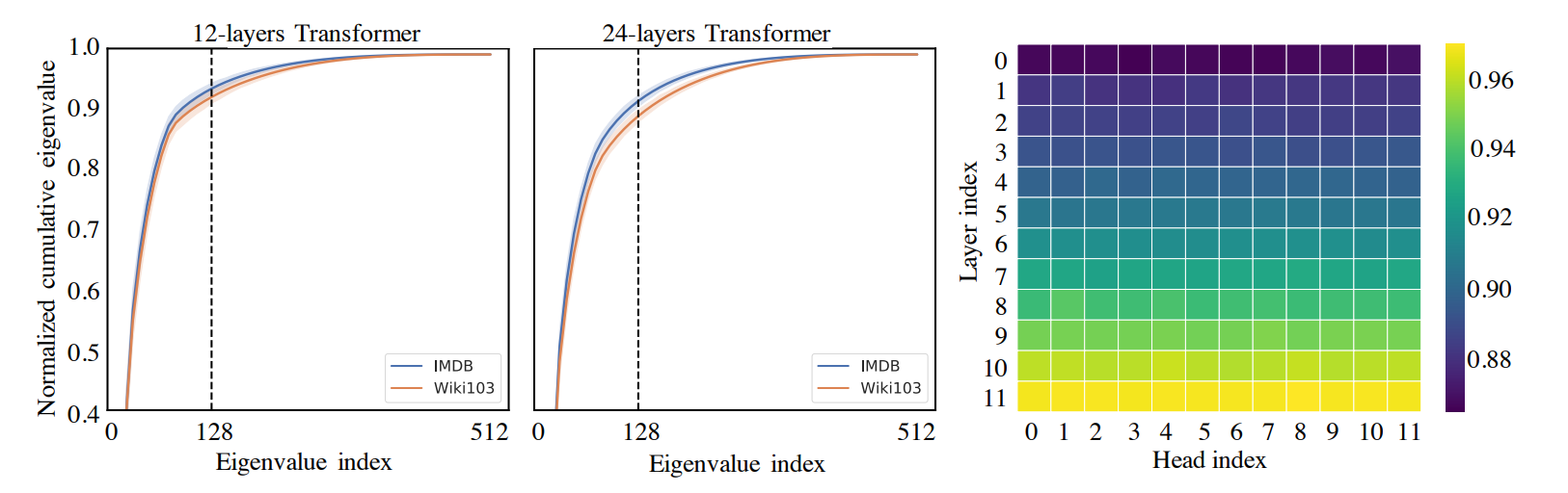
Linformer was perhaps the first paper which used the above observation to linearize self-attention. Suppose we represent $\text{softmax}\left( \frac{QK^T}{\sqrt{d}} \right)$ as $P$. The authors first made empirical investigations which suggest that $P$ is low-rank. (Note that $P$ is not guaranteed to be low-rank since it includes the softmax operation on the low-rank $QK^T$ matrix). In the following figure taken from the paper, we can see that most of the information in $P$ is concentrated in a few eigenvalues, as suggested by the steep cumulative sum curve. Furthermore, the deeper the layer, the lower is the empirical rank of the self-attention matrix, as seen in the figure on the right.
The authors then used the Johnson–Lindenstrauss lemma to claim that there exists a low-rank matrix $\tilde{P}$ which can approximate $P$ with very low error. Intuitively, this works because when computing the self-attention matrix, we are only interested in the pairwise distances between points. The JL-lemma simply says that:
If we use a random projection matrix to project a set of points onto a lower dimension, the pairwise distances are approximately preserved.
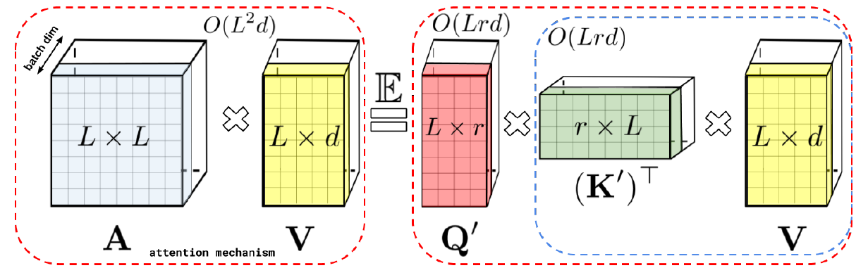
To put theory into practice, the authors projected $K$ and $V$ using a $k\times n$ projection matrix to obtain $\tilde{K}$ and $\tilde{V}$. The product $QK^T$ is now of order $n\times k$, and the final output is still $n\times d$. The Linformer architecture is shown below:
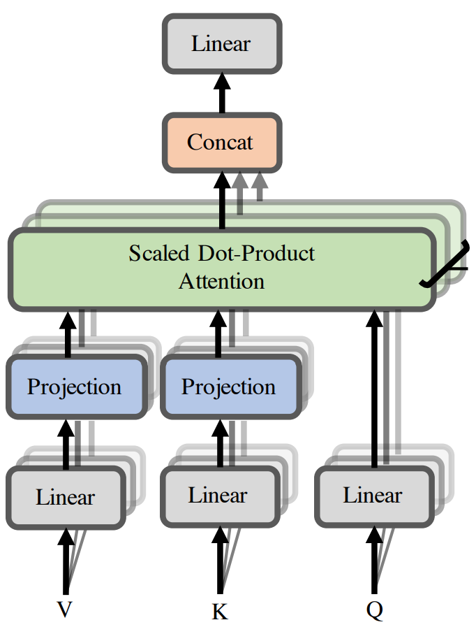
The only remaining question is how to choose an appropriate $k$. Theorem 2 in the paper suggests $k=\Theta(d\log d)$, and proves that for this choice of $k$, there exists projection matrices for which the low-rank approximation holds.
Nystromformer: a Nystrom-based algorithm for approximating self-attention
This paper also uses the low-rank observation, but instead of using JL projections, it uses the Nystrom approximation for approximating $P$. Suppose $P$ is approximately of rank $m$, where $m < n$. Then, we can approximate $P$ with the following matrix:
\[\tilde{P} = \begin{bmatrix} A & B\\ F & FA^+B \end{bmatrix} = \begin{bmatrix}A\\F\end{bmatrix} A^{+} \begin{bmatrix}A & B\end{bmatrix},\]where $A$ is an $m\times m$ matrix consisting of $m$ rows of $P$ (where the rows are chosen according to some scheme), and $A^{+}$ is the Moore-Penrose pseudoinverse of $A$. Each of the computations is now with lower-dimensional matrices linear in $n$. However, there is a caveat: to compute $A$, we still need to first compute $P$, because of the softmax operation (elements of $A$ are normalized by the sum of the entire row in $P$). This defeats the purpose of the approximation, since we were doing it in the first place to avoid computing $P$.
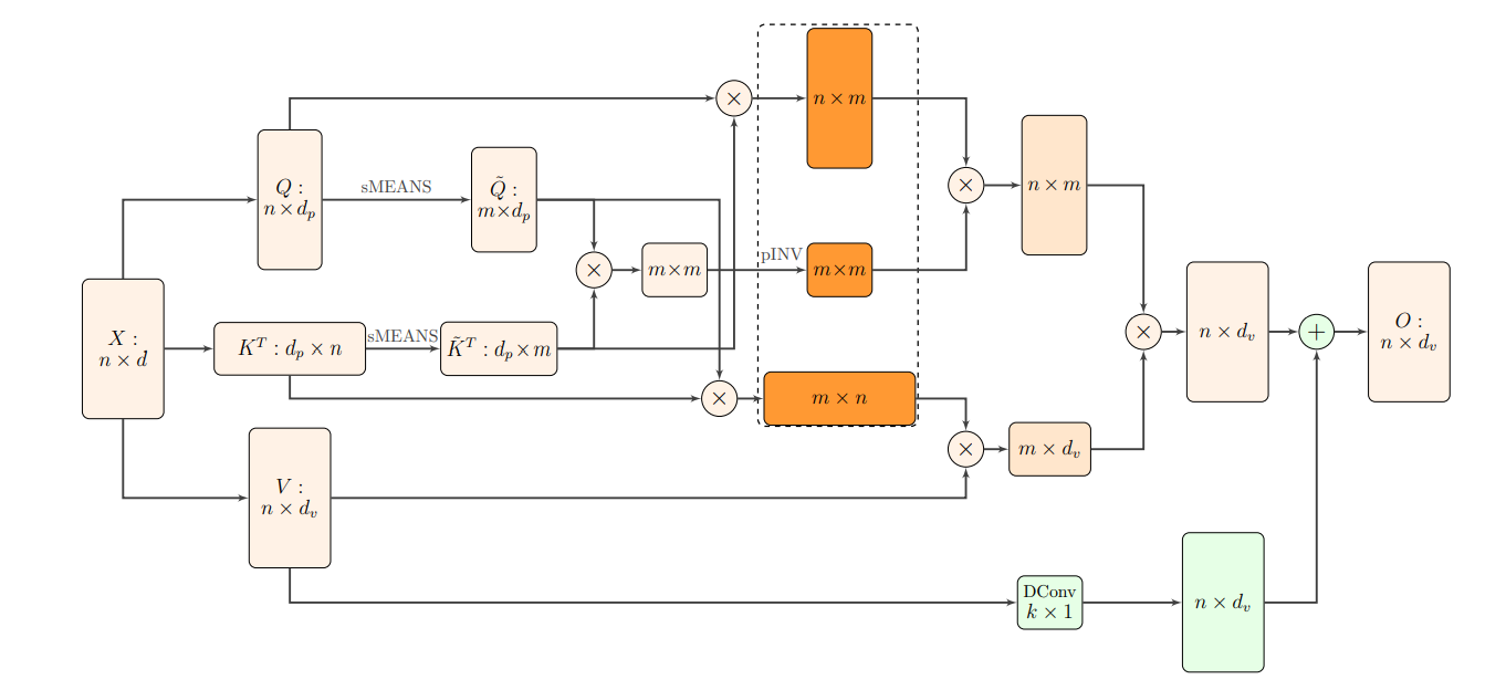
The workaround suggested in the paper is to perform the approximation inside the softmax, and then apply the softmax operation on the approximated matrix. In summary, suppose $\tilde{Q}$ and $\tilde{K}$ denote the $m$-rows of $Q$ and $K$, respectively. Then, the method approximates as follows:
The $m$ rows are formed by using segmental means, i.e., dividing all rows into segments and taking the mean of each segment as a row. The entire computation pipeline of the Nystromformer is shown in the below figure taken from the paper:
Methods based on local-global attention
The second class of methods “sparsifies” attention computation by restricting how many tokens in the sequence each token attends to. Often, such a selection is made using knowledge of the task at hand, i.e., these methods inject some inductive biases into the attention modeling.
Longformer: the long-document transformer
The idea behind longformer can most easily be understood from the following figure taken from the paper:
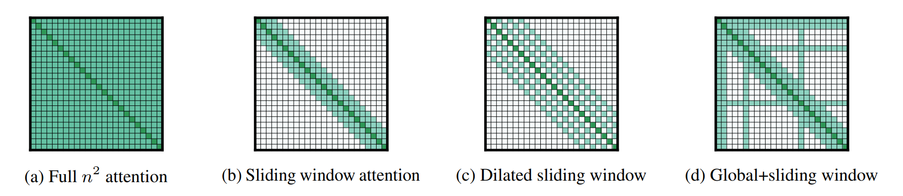
Figure (a) shows the self-attention pattern in the standard transformer. If we restrict each item to only attend to a window of size $w$, this is the windowed attention pattern in (b). It is similar to convolutions, and hence suffers from lack of global context. The context can be extended without increasing computation by using a dilated attention, as in figure (c). The actual longformer uses task-specific global attention in addition to windowed or dilated attention in each layer, as shown in (d). The elements which get this “global” attention are chosen based on the task — for example, the [CLS] token is used for global attention in classification tasks, while for QA, all the question tokens receive global attention.
An important detail in the Longformer paper is the implementation of such an attention pattern. The authors provide a custom CUDA kernel to implement such “banded” matrix multiplication, since it cannot be naturally implemented using existing functions in PyTorch or Tensorflow. Their implementation is available here.
Big Bird: transformers for longer sequences
The core idea of BigBird is very similar to the Longformer, and is shown in the figure below, taken from the paper:
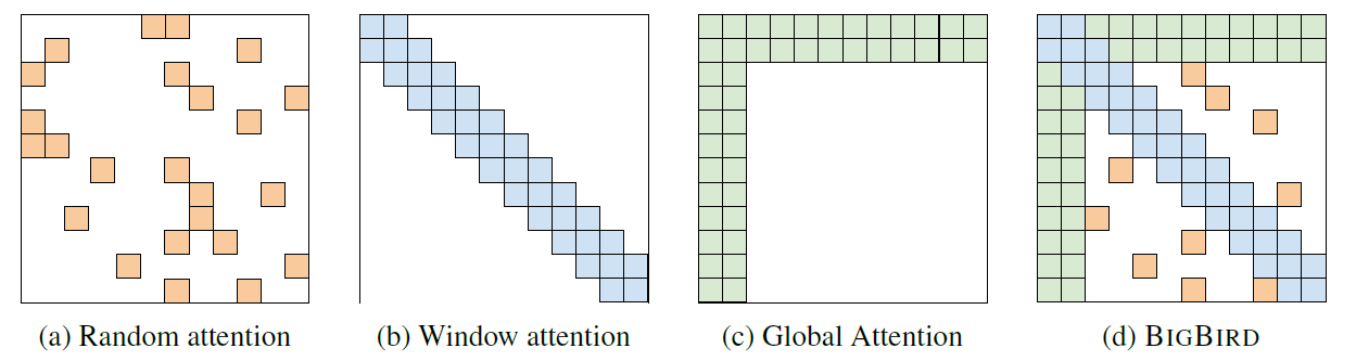
Similar to the longformer, BigBird uses a windowed attention and a selective global attention. Additionally, it also uses a “random attention”, where each token in the sequence attends to a few randomly selected tokens (in addition to the global tokens and those in its window). More importantly, the authors show that this attention pattern has the same expressivity as standard full self-attention, both theoretically and empirically. In particular, they show 2 main things:
- Sparse attention patterns with some “global” tokens are universal approximators, similar to full attention. For this, they use the idea of a “star graph” (as opposed to a complete graph formed by full attention). The idea is that any information routing can be done through the center node, which is the global token.
- Sparse attention is also Turing complete. However, in some cases, it may require a polynomial number of layers where each layer is linear. This kind of defeats the purpose of linear self-attention.
Overall, the random tokens is what makes BigBird different from Longformer, but it seems these random tokens are not really required for the theoretical guarantees. Moreover, they didn’t use the random tokens in their BigBird-ETC experiments either (see Table 8 in the Appendix). One neat trick in the paper is the use of matrix rolling for efficient attention computation, explained in detail in Appendix D.
Long-short transformer: efficient transformers for language and vision
This paper combines a short-term attention and a long-range attention. Their short-term attention is simply the sliding window attention pattern that we have seen previously in Longformer and BigBird. The long-range attention is similar to the low-rank projection idea that was used in Linformer, but with a small change. In Linformer, the key and value matrices $K$ and $V$ were projected using a projection matrix $P \in \mathbb{R}^{n\times r}$ that was learned in training, and was the same for all sequences. In this paper, the matrix $P$ is “dynamic”, and depends on the keys $K$ as $P = \text{softmax}(KW^P)$, where $W^P$ is a $d\times r$ matrix with learnable parameters. This means that a different projection matrix is used for each sequence, and the authors claim that this makes it more robust to insertions, deletions, paraphrasing, etc. The short-term and long-range attentions are then concatenated through a dual layernorm (to rescale them) to obtain the final attention matrix. This entire mechanism is shown in the following figure taken from the paper:
![]()
Methods using softmax as a kernel
Both the categories we have seen previously used some prior inductive biases about the model. The low-rank approximation methods relied on the empirical observation that the self-attention matrix is approximately low rank, while the local-global attention was based on the idea that only a few tokens (often defined based on the task) need to attend globally to all tokens. In contrast, kernel-based approximations do not usually involve any such priors, and as a result, are more mathematically robust. To understand this category of linear transformers, let us take another look at self-attention.
\[SA(Q,K,V) = \text{softmax}\left( \frac{QK^T}{\sqrt{d}} \right)V\]In the above equation, the $SA$ function transformers $Q$, $K$, and $V$ into a sequence of output tokens, say $V’$. We can also write this equivalently as
\[V_i^{\prime} = \frac{\sum_{j=1}^{N}\text{sim}(Q_i,K_j)V_j}{\sum_{j=1}^N \text{sim}(Q_i,K_j)},\]where $ \text{sim}(Q_i, K_j) = \frac{\text{exp}(Q_iK_j)}{\sqrt{d}}.$ Here sim is just a similarity function between query $i$ and key $j$, and we can choose any kernel function for this purpose. Usually, in machine learning, kernel functions are used to avoid explicitly computing coordinates in high-dimensions, but in this case, we will use them in the other direction.
Since $\text{sim}$ is a kernel, there exists some mapping $\phi$ such that
\[\text{sim}(Q_i, K_j) = \phi(Q_i)^T \phi(K_j).\]Using the above decomposition, we can rewrite $ V_i^{\prime}$ as
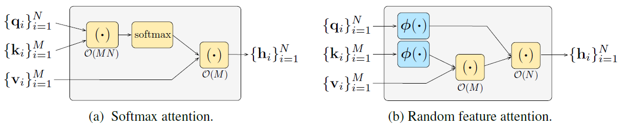
\[V_i^{\prime} = \frac{\sum_{j=1}^{N}\phi(Q_i)^T \phi(K_j) V_j}{\sum_{j=1}^N \phi(Q_i)^T \phi(K_j)}.\]Now, we can take $\phi(Q_i)^T$ outside the summation to get:
\[V_i^{\prime} = \frac{\phi(Q_i)^T \left(\sum_{j=1}^{N} \phi(K_j) V_j\right)}{\phi(Q_i)^T \left(\sum_{j=1}^N \phi(K_j)\right)}.\]The expressions in the parentheses can be computed once and used for all $Q_i$’s — this makes the attention computation linear. Now, the only question is: how do we find such a mapping $\phi$? Unfortunately, the $\phi$ for the softmax kernel is infinite-dimensioal, and so we cannot compute it exactly! The papers in this section use the above idea and try to approximate $\phi$ as best as possible.
Transformers are RNNs: Fast autoregressive transformers with linear attention
In this paper, the authors (somewhat arbitrarily) selected $\phi(x) = \text{elu}(x) + 1$, since this choice results in a positive similarity function. They claim from their experiments that this choice of mapping is on par with the full transformer.
The other important part of the paper (which gives it the name “Transformers are RNNs”) shows an equivalance between autoreressive linear transformers and RNNs. In general, for problems requiring autoregressive computation, a causal masking function is usually employed to compute attention. It can then be shown through an appropriate manipulation of the linear self-attention equation, that the model simply updates an internal states and passes it forward, which should make it equivalent to an RNN.
In any case, this paper was perhaps the first to make the kernel interpretation for softmax attention, and paved the way to more rigorous approximation using random features, which we will see in the next 2 papers. The authors also provide a fast implementation (using gradient computation in CUDA) and an autoreressive generation demo which works on the browser, demonstrating the capabilities of their model.
Rethinking attention with performers
Performers use something called fast attention via positive orthogonal random features, abbreviated as FAVOR+, a method which (the authors claim) can be used for any general-purpose scalable kernel approximation. FAVOR+ is based on the idea of random Fourier features first made popular in this award-winning paper from Rahimi and Recht. The authors propose that any kernel function can be approximated using the following mapping function:
\[\phi(x) = \frac{h(x)}{\sqrt{m}} \left( f_1(\omega_1^T x), \ldots, f_1(\omega_m^T x), \ldots, f_l(\omega_1^T x), \ldots, f_l(\omega_m^T x) \right).\]Here, $\omega$’s are random vectors drawn from some distribution (usually a Normal distribution), $h$ is some function of $x$, and $f_1, \ldots, f_l$ are appropriately chosen deterministic functions. In the original fourier features work, these were often sinusoidal functions (hence the name fourier). $m$ is a hyperparameter which pertains to the accuracy of approximation, i.e., higher the $m$, better the approximation. It turns out that the softmax kernel can be approximated by choosing $h(x) = \text{exp}\left(\frac{\lvert x \rvert^2}{2}\right)$, $f_1 = sin$, and $f_2 = cos$. The fast attention and random features in the method’s name comes from this idea. So what about the positive orthoginality?
There is a caveat in the above approximation. While the method provides a good approximation on average, the variance is quite high, especially when the actual value is close to 0. This is because the softmax kernel is always positive, while the above approximation uses sinusoidal functions which may be positive or negative. Since the self-attention matrix is usually sparse in practice, using the above approximation results in a very high variance empirically. To solve this problem, the authors suggest a slightly different approximation, using $h(x) = \frac{1}{\sqrt{2}}\text{exp}\left(-\frac{\lvert x \rvert^2}{2}\right)$, $f_1(x) = e^x$, and $f_2(x) =e^{-x}$, which results in a similarity function which is always positive. In their experiments, they even replace the exp function with ReLU and get better results. Finally, they show that if we choose the $\omega$’s to be exactly orthogal (using Gram-Schmidt orthogonalization or some other method), the variance can be reduced further. These changes result in the positive orthogonal in the name.
Using the above mapping function, $Q$ and $K$ can be mapped to $Q^{\prime}$ and $K^{\prime}$, and the matrix multiplications can be broken down into the following form, which results in linear complexity.
Random feature attention
This paper was published concurrently with the Performer paper at ICLR 2021, and proposes the same idea of approximating the softmax kernel using random features. A similar extension of Rahimi and Recht’s work is used to compute a mapping $\phi$ that approximates the similarity function computed by softmax:
Additionally, this paper also proposes a method for learning with recency bias, since softmax does not explicitly model distance or locality (hence the importance of positional encodings in transformers). In the “transformers are RNNs” paper, we saw how autoregressive transformers can be shown to be equivalent to RNNs. Inspired from this equivalence, the authors in this paper further add a learned gating mechanism in the computation which biases the model to rely more on recent tokens.
Summary
Here is a tabular summary of all the papers covered in this post:
| Method Name | Concept used | Approximation method | Implementations |
|---|---|---|---|
| Linformer | Low-rank approximation | JL projection matrices | Original (Fairseq), PyTorch |
| Nystromformer | Low-rank approximation | Nystrom approximation | Original, PyTorch |
| Longformer | Local-global attention | Window + Task-specific global attention | Original, HuggingFace |
| Big Bird | Local-global attention | Window + global + block-wise random | Original (Tensorflow), HuggingFace |
| Long-short transformer | Local-global attention | Window + dynamic JL projection matrix | PyTorch |
| Fast transformer | Softmax kernel | $\phi(x) = \text{elu}(x) + 1$ | Original, Reimplementation |
| Performer | Softmax kernel | FAVOR+ | Original (TF), PyTorch, HuggingFace |
| Random Features Attention | Softmax kernel | Random features + gating |
I hope this summary would be useful to keep track of all the research happening in the field of efficient transformers.