Recently, I have been involved in several projects related to speaker diarization. For the uninitiated, diarization is defined as the task of partitioning a recording into homogeneous speaker segments — which is just a fancy way of saying “who spoke when”.
For example, suppose you have a 1-hour meeting recording where Marie, Abhishek, Mitchell, and Jinyi participated. The desired output should divide the recording into segments, and each segment should be tagged with a speaker label. Importantly, it is NOT required to provide absolute speaker identities, since that would need the system to know all the possible speakers in advance. What this means is that your output can contain labels A, B, C, and D, and it is incumbent upon the evaluation system to then assign these to the original speaker IDs in such a way that minimizes the final error rate. For example, the evaluation may decide that the best error rate is obtained by mapping (Marie, B), (Abhishek, C), (Mitchell, A), and (Jinyi, D).
Formally, a diarization system produces a set of segment-label tuples of the form (start time, end time, speaker). In the following, we will use the terms “reference” and “hypothesis” to refer to the ground truth and the diarization system output, respectively.
For tasks such as image classification or speaker verification, where the output is a single label, evaluation is relatively simple. However, evaluating sequence-based tasks is relatively harder. In speech recognition, for instance, you are required to compute the Levenshtein edit distance between two word sequences, which involves solving a dynamic programming problem. Machine translation evaluation is even more challenging, since monotonicity of sequences is lost. Similarly, diarization evaluation requires finding an optimal speaker assignment, and then counting matching speakers within each region (as we will see next). This requires solving a linear sum assignment problem, sorting the reference and hypothesis lists, and iterating over them multiple times, all of which contributes to computation time. This means that if you are evaluating your diarization system on a dataset which contains hour-plus recordings (or even day-long recordings as is common for child language acquisition data) comprising frequent turn-taking between speakers, computing DER itself may take several minutes. (This is, of course, negligible compared to neural networks which train for weeks, but we should cut cost and complexity wherever possible.)
I will briefly describe how we compute Diarization Error Rate (DER), the most popular metric for evaluating diarization systems. The equations are well known, but here I have borrowed them from Xavier Anguera’s thesis.
How DER is computed
Suppose we have found an optimal mapping between all the reference and hypothesis speakers. (It is likely that they differ in the number of speakers in which case some speakers will be left unmapped.)
The reference and hypothesis lists are taken together and collapsed, and we get “regions” between each time mark, where a time mark may be either a start or an end time. The idea is that within each region, speakers are consistent, i.e., there is no speaker change. Suppose each such region is denoted by $r$. Let $\text{dur}(r)$ denote the duration of the region, and $N_{ref}$ and $N_{hyp}$ denote the number of reference and hypothesis speakers, respectively, in region $r$ (each of these may be greater than 1 since overlapping speech may be present in the recording). For each region, let $N_{cor}$ be the number of speakers in this region that are correctly matched between the reference and hypothesis. For example, if the reference says Marie and Mitchell are speaking in the region, while the hypothesis just has label A for the region, $N_{cor} = 1$.
We then compute the following 3 quantities:
- Missed speech: It is the fractional duration of speaking time in the reference which is not accounted for in the hypothesis:
Intuitively, the numerator computes the total speaker time which is missed by the hypothesis, and the denominator computes the total reference speaker time in the recording. Note that this is not the same as the recording duration. For example, for a 100s recording with 40% overlapping speech (2 speaker overlaps), the total speaking time would be 140s.
- False alarm: It is the fractional duration of speaking time that is extra in the hypothesis, i.e., which is labeled non-speech in the reference:
Again, the numerator computes the total false alarm speaking time, and the denominator gives the total speaking time.
- Speaker confusion: It is the fractional duration of speaking time in which the hypothesis assigns the wrong speaker label:
It is easy to understand by observing that the difference in the numerator would give us the number of incorrect speakers assigned in that particular region.
Once we have these quantities, DER is simply given as the sum: $\text{DER} = E_{miss} + E_{falarm} + E_{conf}$.
While DER is the most popular metric for evaluating diarization systems, it is certainly not the only one. Recently, the DIHARD challenges have also measured a metric called Jaccard Error Rate (JER) through the dscore toolkit. JER is based on Jaccard index, which computes the “intersection-over-union” of two sets. For the purpose of diarization, JER is computed as 1 minus the average of Jaccard indices for all reference-hypothesis speaker pairs.
Correlation between DER and other metrics such as JER is still an open problem. In this post, I will focus on DER since it is most widely reported in all diarization research.
Tools for computing DER
Now that we know how DER is conceptually computed, I will mention widely used implementations of this metric.
-
md-eval.pl: Oddly enough, the most popular tool for evaluating diarization systems is a 3000-line Perl script from NIST called md-eval.pl. It is easy to use from the command line, and choke full of features.
-
dscore: To compute DER,
dscoreprovides a Python wrapper around md-eval.pl, and then uses regular expressions to extract the relevant information from the stdout. Additionally,dscorealso provides a number of other metrics, including JER. -
pyannote.metrics: It is part of the
pyannotetoolkit, which provides easy end-to-end diarization pipelines. The DER computation is implemented in Python, and the optimal speaker mapping usesscipy.optimize.linear_sum_assignment(there is also an option for “greedy” assignment). The DER function can directly be called from Python without the need to write them out to files, unlikemd-evalanddscore. The toolkit provides a set of other metrics such as cluster purity and coverage. -
simpleder: It is a lightweight library which computes DER by summing the costs from the optimal assignment, which are obtained using
scipy.optimize.linear_sum_assignment. While the package is easy-to-use and fast, its major limitation is that it cannot handle overlapping speech.
The problem
Suppose you are working on a Python-based (as is common now) pipeline which requires you to compute the DER between a reference and hypothesis list of turns. If you know that the turns do not overlaps, simpleder is arguably the easiest option to do it. Otherwise, you have 2 options:
- Write the turns out to files (on your filesystem or in the buffer memory), run
md-eval.pl, and parse the stdout output using regex to extract the relevant metrics.- Pros: fast, easy installation
- Cons: complicated parsing, not very Pythonic
- Invoke the
pyannote.metricsDER computation function directly from your Python program.- Pros: easy to use
- Cons: slower than md-eval, installs several dependencies
We will see how to do both later in this post.
While working on DOVER-Lap, I needed to quickly compute the DER between all pairs of input hypotheses (to implement the DOVER label mapping). I first tried md-eval.pl, and while that was relatively fast, it added a dependency on an external script, and was not very Pythonic in terms of packaging. It requires invoking a subprocess and using complicated regular expressions (which I borrowed from the dscore toolkit), all of which is not particularly elegant. Next, I installed pyannote.metrics, but it turned out to be almost 10 times slower than md-eval (when using the optimal mapping). (Note: This is not to say that pyannote.metrics is bad. The entire pyannote library provides some very easy-to-use pipelines, and we even used its overlap detection pipeline in our Hitachi-JHU DIHARD3 submission. “Slow” here means, for example, you wouldn’t install Kaldi if all you needed was to compute word error rates.) I started looking around for a small, fast, easy-to-use package which computes DER between lists of turns. simpleder immediately looked promising, until I saw that it couldn’t handle overlaps.
Eventually, I took it upon myself to implement such a package, which would simply compute DER fast: DO ONE THING, DO IT WELL.
Spyder: a simple Python package for fast DER computation
First steps
I started with the simpleder library as template, and extended it such that it could handle overlapping segments. This sounds simple enough, but the computation becomes completely different. Without overlaps, it suffices just to sum the optimal mapping cells in the linear sum assignment table. However, once overlaps are present, we must iterate through all regions of the collapsed reference and hypothesis, and keep adding to the metrics as I described through the equations earlier.
This directly introduces additional computational costs, proportional to the number of such “regions”. There are additional costs to map old speaker labels to new labels, keep track of running speakers across regions, and so on. When I had an initial Python implementation in place, I found that I was still much slower than md-eval (although reasonably faster than pyannote.metrics).
Small improvements
Since I was not happy with the processing speed, I tried various things to speed it up:
- I replaced
scipy.optimize.linear_sum_assignmentwith lapsolver for computing the optimal speaker mapping. This only made a small difference since our matrices are often quite small (e.g., 5x5 for 5 speaker recordings). - More importantly, I used Cython to compile the Python script into C binaries, which immediately resulted in a 2x speed-up.
Cython was a game-changer, and 1 entire weekend, I messed around reading blog posts on Cythonizing Python code, and implementing the suggestions in my code. I added C type definitions, defined function types, and kept making tweaks until the code was barely recognizable as Python anymore. However, all of these changes only gave me a small speed-up over what I already had from simple compilation. I knew it was time for a major code overhaul.
The big leap
Perhaps a better Python programmer would have been able to implement my DER computation code to run close to a native C++ implementation, but it is unlikely. There’s a reason why all high-performance libraries are written in C++. Especially for my case, since I wanted to iterate over lists of tuples containing different primitive types, the Python code introduced overheads since it needs to store the types along with each object. (It’s also interpreted rather than compiled, but I was already dealing with that constraint using Cython.)
Anyway, I decided to re-implement my code in pure C++, and then provide a Python interface using pybind11. (I had another interest in pursuing this direction: my advisor Dan Povey’s new project K2 is written in C++ with pybind11 for interfacing, so I wanted to get familiar with the tool.)
Since I had committed to the big leap, the next obvious simplification was to have an in-house implementation of the Hungarian algorithm for optimal mapping, instead of relying on external tools. The motivation behind this is that most of these libraries are designed for high-performance on large matrices, but don’t really provide much for smaller cases as is common in our task. Luckily, I found an excellent C++ implementation of the Hungarian algorithm with a BSD license, and I borrowed the code directly into my module (with minor changes to perform maximization instead of minimization). The rest of the implementation was also quite streamlined, once I had the basic classes and functions in place. (I also learnt to appreciate the importance of header files during this time.)
It took me another day to implement the pybind11 interfaces, which turned out to be really simple in the end. Eventually, I had spyder, which is a play on a “simple Python package for fast DER computation”. Preliminary experiments suggested that this implementation was 10x faster than my original Python implementation. It is:
- blazingly fast
- stand-alone (as in zero dependencies)
- easy-to-use (from both Python code and the terminal)
Benchmarking DER computation speed with Spyder
In the rest of this blog post, I will benchmark the computation speeds of md-eval.pl and pyannote.metrics, and compare them with spyder. For this purpose, I am using the popular AMI meeting corpus. In particular, I will be using the development set, which contains 18 recordings. For our hypothesis, I will use the output from an overlap-aware spectral clustering system that I presented at IEEE SLT 2021.
Let us first load the reference and hypothesis turns.
from collections import defaultdict

REF_FILE = 'ref_rttm'
HYP_FILE = 'hyp_rttm'

def load_rttm(file):
    rttm = defaultdict(list)
    with open(file, 'r') as f:
        for line in f:
            parts = line.strip().split()
            file_id = parts[1]
            spk = parts[7]
            start = float(parts[3])
            end = start + float(parts[4])
            rttm[file_id].append((spk, start, end))
    return rttm

ref_turns = load_rttm(REF_FILE)
hyp_turns = load_rttm(HYP_FILE)
len(ref_turns.keys())
18
import numpy as np

total_spk_duration = {
    key:sum([turn[2]-turn[1] for turn in ref_turns[key]]) for key in ref_turns
}
x = np.array(list(total_spk_duration.values()))
f'Average duration = {x.mean()}, std: {x.std()}'
'Average duration = 1971.9567222222229, std: 660.7636193357241'
num_turns = {key:len(ref_turns[key]) for key in ref_turns}
y = np.array(list(num_turns.values()))
f'Average # of turns = {y.mean()}, std: {y.std()}'
'Average # of turns = 537.5555555555555, std: 219.56401805553512'
So we have 18 recordings of average duration 0.55 hours, with an average of 537 turns per recording. Later, we will visualize the DER computation in terms of duration and frequency of turn taking. Let us now write functions to compute DER using each tool. We will use the following generic function to time each function.
import time

def compute_der_and_time(ref_turns, hyp_turns, der_func):
    ders = {}
    times = {}
    for reco in ref_turns:
        ref = ref_turns[reco]
        hyp = hyp_turns[reco]
        start_time = time.time()
        der = der_func(ref, hyp)
        end_time = time.time()
        ders[reco] = der
        times[reco] = (end_time - start_time)*1000
    return ders, times
Scoring with md-eval.pl
# We have the md-eval.pl file in the same directory
import os
import shutil
import subprocess
import tempfile

MDEVAL_BIN = os.path.join(os.getcwd(), 'md-eval.pl')

def write_rttm(file, turns):
    with open(file, 'w') as f:
        for turn in turns:
            f.write(f'SPEAKER reco 1 {turn[1]} {turn[2]-turn[1]} <NA> <NA> {turn[0]} <NA> <NA>\n')

def DER_mdeval(ref_turns, hyp_turns):
    tmp_dir = tempfile.mkdtemp()

    # Write RTTMs.
    ref_rttm_fn = os.path.join(tmp_dir, 'ref.rttm')
    write_rttm(ref_rttm_fn, ref_turns)
    hyp_rttm_fn = os.path.join(tmp_dir, 'hyp.rttm')
    write_rttm(hyp_rttm_fn, hyp_turns)

    # Actually score.
    try:
        cmd = [MDEVAL_BIN,
               '-r', ref_rttm_fn,
               '-s', hyp_rttm_fn,
              ]
        stdout = subprocess.check_output(cmd, stderr=subprocess.STDOUT)
    except subprocess.CalledProcessError as e:
        stdout = e.output
    finally:
        shutil.rmtree(tmp_dir)

    # Parse md-eval output to extract overall DER.
    stdout = stdout.decode('utf-8')
    for line in stdout.splitlines():
        if 'OVERALL SPEAKER DIARIZATION ERROR' in line:
            der = float(line.strip().split()[5])
            break
    return der
der_mdeval, time_mdeval = compute_der_and_time(ref_turns, hyp_turns, DER_mdeval)
for key in der_mdeval:
    print(f'{key}: DER={der_mdeval[key]}, Time={time_mdeval[key]:.2f}')
ES2011a.Mix-Headset: DER=32.99, Time=85.05
ES2011b.Mix-Headset: DER=18.9, Time=71.56
ES2011c.Mix-Headset: DER=24.29, Time=76.52
ES2011d.Mix-Headset: DER=42.69, Time=102.03
IB4001.Mix-Headset: DER=28.09, Time=91.80
IB4002.Mix-Headset: DER=48.21, Time=115.40
IB4003.Mix-Headset: DER=17.6, Time=77.12
IB4004.Mix-Headset: DER=23.14, Time=106.63
IB4010.Mix-Headset: DER=21.93, Time=140.51
IB4011.Mix-Headset: DER=19.28, Time=116.78
IS1008a.Mix-Headset: DER=11.14, Time=45.12
IS1008b.Mix-Headset: DER=13.81, Time=58.98
IS1008c.Mix-Headset: DER=20.18, Time=66.28
IS1008d.Mix-Headset: DER=21.46, Time=69.06
TS3004a.Mix-Headset: DER=31.22, Time=71.98
TS3004b.Mix-Headset: DER=21.97, Time=99.36
TS3004c.Mix-Headset: DER=18.85, Time=121.24
TS3004d.Mix-Headset: DER=28.81, Time=137.14
Scoring with pyannote.metrics
from pyannote.metrics.diarization import DiarizationErrorRate
from pyannote.core import Annotation, Segment

def DER_pyannote(ref_turns, hyp_turns):
    ref = Annotation()
    for turn in ref_turns:
        ref[Segment(start=turn[1],end=turn[2])] = turn[0]
    hyp = Annotation()
    for turn in hyp_turns:
        hyp[Segment(start=turn[1],end=turn[2])] = turn[0]
    metric = DiarizationErrorRate()
    return metric(ref, hyp)
der_pyannote, time_pyannote = compute_der_and_time(ref_turns, hyp_turns, DER_pyannote)
/Users/desh/opt/miniconda3/envs/spyder/lib/python3.7/site-packages/pyannote/metrics/utils.py:184: UserWarning: 'uem' was approximated by the union of 'reference' and 'hypothesis' extents.
  "'uem' was approximated by the union of 'reference' "
for key in der_mdeval:
    print(f'{key}: DER={100*der_pyannote[key]:.2f}, Time={time_pyannote[key]:.2f}')
ES2011a.Mix-Headset: DER=33.04, Time=232.07
ES2011b.Mix-Headset: DER=18.90, Time=276.72
ES2011c.Mix-Headset: DER=24.42, Time=384.01
ES2011d.Mix-Headset: DER=42.73, Time=748.00
IB4001.Mix-Headset: DER=28.04, Time=660.65
IB4002.Mix-Headset: DER=48.22, Time=1018.05
IB4003.Mix-Headset: DER=17.56, Time=404.99
IB4004.Mix-Headset: DER=23.13, Time=883.88
IB4010.Mix-Headset: DER=21.97, Time=1603.37
IB4011.Mix-Headset: DER=19.57, Time=986.38
IS1008a.Mix-Headset: DER=10.84, Time=84.62
IS1008b.Mix-Headset: DER=13.81, Time=207.91
IS1008c.Mix-Headset: DER=20.42, Time=277.53
IS1008d.Mix-Headset: DER=21.42, Time=333.36
TS3004a.Mix-Headset: DER=31.05, Time=357.73
TS3004b.Mix-Headset: DER=21.99, Time=716.02
TS3004c.Mix-Headset: DER=19.01, Time=1055.47
TS3004d.Mix-Headset: DER=29.03, Time=1572.22
Scoring with Spyder
import spyder

def DER_spyder(ref_turns, hyp_turns):
    der = spyder.DER(ref_turns, hyp_turns).der
    return der
der_spyder, time_spyder = compute_der_and_time(ref_turns, hyp_turns, DER_spyder)
for key in der_spyder:
    print(f'{key}: DER={100*der_spyder[key]:.2f}, Time={time_spyder[key]:.2f}')
ES2011a.Mix-Headset: DER=32.99, Time=6.82
ES2011b.Mix-Headset: DER=18.90, Time=8.45
ES2011c.Mix-Headset: DER=24.29, Time=11.80
ES2011d.Mix-Headset: DER=42.69, Time=22.80
IB4001.Mix-Headset: DER=28.09, Time=18.65
IB4002.Mix-Headset: DER=48.21, Time=31.99
IB4003.Mix-Headset: DER=17.60, Time=10.95
IB4004.Mix-Headset: DER=23.14, Time=24.95
IB4010.Mix-Headset: DER=21.93, Time=43.87
IB4011.Mix-Headset: DER=19.28, Time=30.81
IS1008a.Mix-Headset: DER=11.14, Time=2.22
IS1008b.Mix-Headset: DER=13.81, Time=5.54
IS1008c.Mix-Headset: DER=20.18, Time=7.92
IS1008d.Mix-Headset: DER=21.46, Time=9.03
TS3004a.Mix-Headset: DER=31.22, Time=10.77
TS3004b.Mix-Headset: DER=21.97, Time=21.25
TS3004c.Mix-Headset: DER=18.85, Time=30.75
TS3004d.Mix-Headset: DER=28.81, Time=49.40
mdeval = sum(list(time_mdeval.values()))/len(time_mdeval)
pyannote = sum(list(time_pyannote.values()))/len(time_pyannote)
spyder = sum(list(time_spyder.values()))/len(time_spyder)

print (f"Average DER computation time per file:")
print (f"md-eval: {mdeval:.2f} ms")
print (f"pyannote: {pyannote:.2f} ms")
print (f"spyder: {spyder:.2f} ms")
Average DER computation time per file:
md-eval: 91.81 ms
pyannote: 655.72 ms
spyder: 19.33 ms
We can see that Spyder is almost 4-5x faster than md-eval, and at least 10x faster than Pyannote. Note that this is not particularly fair for Pyannote, since creating Segments and Annotations from the list of turns initializes several things which can be used to compute different metrics. However, for a straight-forward DER computation, these can be considered overhead. Spyder also initializes a TurnList class which is a C++ vector of Turn types, but this initialization is much faster, perhaps because of defined object types.
How does recording duration or number of turns affect DER computation speed?
Let us now plot the computation times as functions of recording duration, and number of turns.
# Duration vs speed
import matplotlib.pyplot as plt
plt.rcParams['figure.figsize'] = [10, 6]
plt.rcParams['figure.dpi'] = 100 # 200 e.g. is really fine, but slower

plt.scatter(x, list(time_mdeval.values()), marker='o', label='md-eval')
plt.scatter(x, list(time_pyannote.values()), marker='^', label='pyannote')
plt.scatter(x, list(time_spyder.values()), marker='d', label='spyder')
plt.legend(loc='best')
plt.yscale('log')
plt.xlabel('Recording duration (s)')
plt.ylabel('Time (ms)')
plt.show()
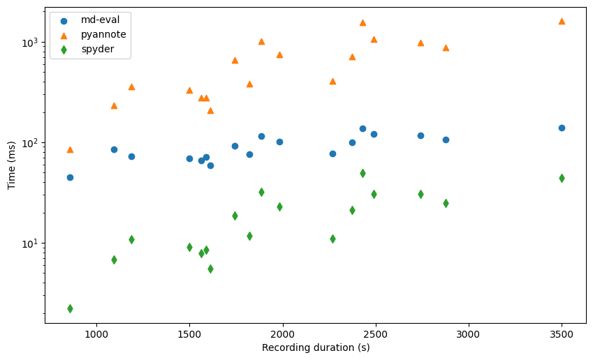
For convenience, we have plotted the y-axis in the log domain so that the systems are well separated.
We see that there is a positive correlation between the recording duration and the computation time, especially for pyannote and spyder. For md-eval, most of the time seems to be taken by I/O so that the actual processing time does not matter.
# No. of turns vs speed

plt.scatter(y, list(time_mdeval.values()), marker='o', label='md-eval')
plt.scatter(y, list(time_pyannote.values()), marker='^', label='pyannote')
plt.scatter(y, list(time_spyder.values()), marker='d', label='spyder')
plt.legend(loc='best')
plt.yscale('log')
plt.xlabel('Number of turns')
plt.ylabel('Time (ms)')
plt.show()
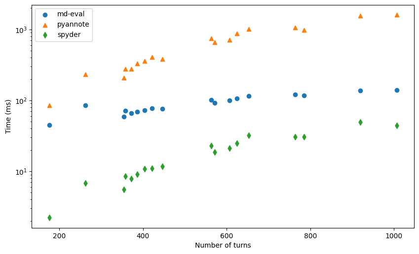
We again find a very strong correlation, as expected. DER computation requires iterating over the turns list, so it increases with increase in number of turns.
Concluding thoughts
We saw how DER is computed, and the popular tools to compute it given reference and hypothesis list of turns. We enumerated some of the limitations with existing tools for evaluating diarization systems, and saw how Spyder can address some of these. Its major advantages are:
- Fast: Implemented in pure C++, and faster than the alternatives (md-eval.pl, dscore, pyannote.metrics). It is about 4-5x faster than using a wrapper around md-eval, for instance.
- Stand-alone: It has no dependency on any other library (except
clickfor argument parsing). We have our own implementation of the Hungarian algorithm, for example, instead of usingscipy. - Easy-to-use: No need to write the reference and hypothesis turns to files and read md-eval output with complex regex patterns. Spyder can be used from a Python program as well as from the command line.
- Overlap: Spyder supports overlapping speech in reference and hypothesis.
I had a lot of fun building this small C++/Pybind11 package and hope that people find it useful in their work on diarization.
There is a long way to go still, however. I began writing Spyder to simply do fast DER computation, but with the numerous diarization evaluation metrics out there spread out among several toolkits, it might be useful to have all their (fast) implementations in one place. Over the next few months, I will try to extend Spyder to support all such metrics, in the hope that it eventually becomes the go-to toolkit for diarization evaluation. As always, help in the form of pull requests are welcome!