Understanding the JHU CHiME-6 Submission - Part I (Enhancement)

The CHiME-6 challenge concluded last month and our team from JHU was ranked 2nd in Track 2 (“diarization + ASR” track). For a reader unfamiliar with the challenge, I would recommend listening to the audio samples provided on the official webpage. The data is notoriously difficult for speech recognition systems, as evident from the fact that even after 2 editions of the challenge using the same data, the best achieved WER is still over 30%. This edition had the additional challenge (in Track 2) that teams were not allowed to use oracle speech segments and speaker information, and the evaluation metric was a type of “speaker-attributed” WER. The best scores achieved in this task were close to 45%, meaning that for every 100 words in the reference, 45 were either:

• missed in the hypothesis,
• false alarms,
• substituted for a different word, or
• attributed to a different speaker.

Note that even with a good ASR system, if speaker diarization (“who spoke when”) is not performed well, the metric would output very poor scores. As a result, it was important for teams to do well on the entire pipeline. (Remarkably, the baseline score for track 2 was >80%.) The official webpage contains the 2-page abstracts, slides, and video presentations for all the participating teams.

This post is not an “appendix” to our system description paper. It is more of an attempt to understand the numerous techniques that were used in the entire CHiME-6 pipeline. I find that due to page limitations, papers often reduce an important method to an abbreviation and a reference (e.g., “we used online WPE [4] for dereverberation”, or “we applied GSS [17] using the RTTM file”). As a fairly new speech researcher (less than 2 years in the field), I found that my understanding of these methods is not satisfactory. Therefore, I decided to write a series of posts in which my objective would be to simplify all these mystic method names, while also providing small details of their impact on our system. This will be a 3-part series (similar to our breakdown of the pipeline) comprising the following:

1. Speech Enhancement: dereverberation, beamforming
2. Speaker Diarization: x-vector/clustering system, EEND, overlap-aware VB resegmentation
3. Speech Recognition: GSS, Kaldi chain model, RNNLM

The following figure shows an overview of the pipeline we used for the challenge:

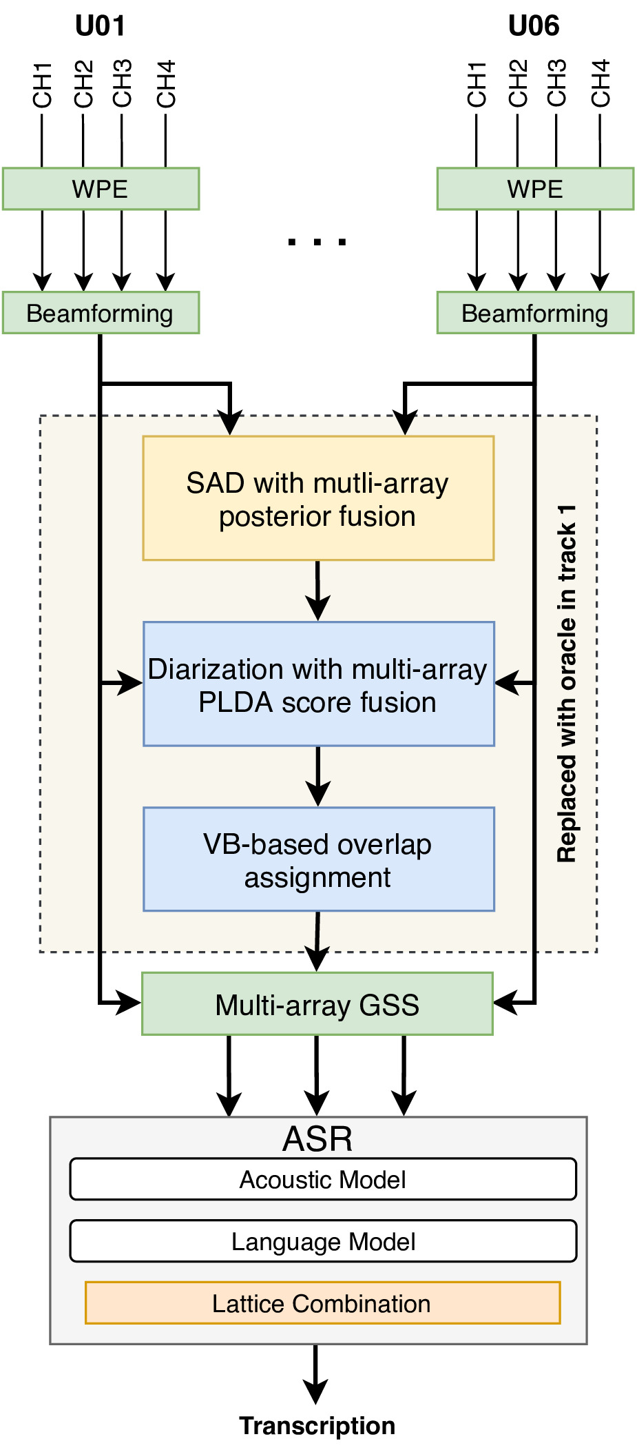
Overview of the JHU CHiME-6 system.

The expectation is that this series will provide the reader a general overview and appreciation of the various sub-tasks and techniques that constitute solving a complex task such as the cocktail party problem. This is especially relevant in the current environment of end-to-end solutions.

The baseline CHiME-6 recipe is publicly available and contains most of the above mentioned components. We are working on a better recipe comprising lessons/methods from the workshop.

NOTE: This series of posts borrows from work done by several members of the JHU CHiME-6 team, including Ashish Arora, Ke Li, Aswin Shanmugam Subramanian, Bar Benyair, and Paola Garcia.

Preliminary

Before we get into the actual system, there is some terminology that you should be familiar with. The CHiME-6 data consists of 20 dinner parties (approximately 1-2 hours each) which is divided into 16/2/2 for train/dev/eval. Each party comprises 4 speakers. The data is collected on biaural headset microphones worn by each participant, and also on 6 Kinect devices placed (2 each) in the living room, dining room, and the kitchen, to obtain simultaneous close-talk and far-field data. Each Kinect device contains 4 microphones, thereby providing 24 channels in total. We call each Kinect device an “array”. Some of the arrays may be faulty in some sessions, and the details are provided here. The key difference between CHiME-5 and CHiME-6 data is that all arrays have been synchronized by Jon Barker. This makes it possible to use several multi-channel techniques. For dev and eval, only far-field array microphones are allowed to be used, but close-talk utterances may be used for training.

Speech Enhancement

Speaker diarization and speech recognition systems are adversely affected by noise and reverberation in a signal. Speech enhancement aims to remove the noise, thereby making it more intelligible for a human listener and also easier to diarize/transcribe for a downstream system. There are 2 key components to enhancement: dereverberation and denoising. As the names suggest, they deal with the removal of reverberation and noise from the signal, respectively. We used a version of WPE for dereverberation and a filter-and-sum beamformer for beamforming at the source, which is discussed next.

Dereverberation using WPE

WPE stands for Weighted Prediction Error¹. I will first describe the offline version of the method proposed in the original paper, and then talk about the online version we used in our system. The following discussion is mostly based on this paper.

WPE is a method for “blind” speech dereverberation, i.e., no training or bias is required for performing the dereverberation. It uses multi-channel linear prediction (MCLP). Suppose we have $M$ channels and the clean speech in each channel is given by STFT coefficients $s_{n,k}^m$, where $n$ and $k$ are time frame index and frequency bin index, respectively. Let $x_{n,k}^m$ denote the actual observed STFT coefficient. We can express the observed coefficient in terms of the clean speech coefficients as

where $h_{l,k}^m$ models the acoustic transfer function (ATF) between the speech source and the microphone $m$, and e_{n, k}^{m} is an additive noise signal (which we can assume to be 0 for now). The ATF can be thought of as an approximation of the combined effect of all the paths between the source and receiver in a room. Let $D$ be the duration of early reflections, and denote

which is the combination of the anechoic (clean) signal, and the early reflections. Note that this quantity is what we want to estimate. We can split the summation term in the first equation into $d_{n,k}^m$ and the residual, which needs to be removed. By replacing the convolutive model with an autoregressive model, we can rewrite the observed signal at $m=1$ as

Here, $\mathbf{g}_{k}^{m}$ is the regression vector of size $L_k$ for the channel $m$, and $(\cdot)^H$ is conjugate transpose. Combining all $x$’s in a vector $\mathbf{x}$, we can write

In WPE, each STFT coefficient of the desired signal is modeled as a zero-mean complex Gaussian random variable (see this Wikipedia article) with a variance $\lambda_{n,k}$. Moreover, all the coefficients are assumed to be independent of each other. Then, we can estimate $\mathbf{g}_k$ and $\lambda_{n,k}$ by maximizing the likelihood

where $\Theta_{k}$ consists of the regression vector and the variances. By taking the negative log of the likelihood, we arrive at the following cost function which needs to be minimized:

The function cannot be solved analytically, so WPE solves it in a two-step iterative process, by alternatively keeping $\mathbf{g}_{k}$ and $\lambda_{n,k}$ fixed and minimizing w.r.t the other. Thus, modeling STFT coefficients using complex Gaussians, and the two-step optimization procedure forms the core of the WPE method for dereverberation.

The official NTT-WPE implementation consists of this iterative method, and they used a context window around the current STFT bin variance, since it was found to improve the estimate. However, this makes the algorithm dependent on future context. This method was recently extended to the online case ² by making the filter coefficients rely only on the causal estimates, thus providing Recursive Least Squares type updates. The NARA WPE³ implementation from Paderborn University provides both offline and online versions, and we used the online WPE in our system.

Beamforming

Denoising using beamforming is the second key element in our enhancement module. In the baseline recipe that we built for the challenge, we used the simple filter-and-sum beamformer⁴ implemented in the BeamformIt toolkit. During the challenge, we also experimented with using a neural beamformer, although this was not included in the final submission. I will describe both of these beamforming methods next.

Filter-and-sum beamformer: This method was first proposed in 2007⁴, and is a very simple technique requiring no mask estimation. My description here is taken from the PhD thesis of Xavier Anguera, who first introduced this method and implemented BeamformIt. (Note: BeamformIt is used in Kaldi for beamforming.)

This beamforming technique is similar to the simpler delay-and-sum method, which I will first summarize. The idea is that if signal from the same source is captured by several receivers, they all have the same waveform, but differ in delay and phase. So, if a different delay is applied to each input signal depending on the location of the microphone, the source signals captured at all the microphones become “in-phase”, and the additive noise will be out of phase. Adding all the signals and normalizing by the number of channels will then remove the noise from the signal. Mathematically, for a linear microphone array consisting of $N$ microphones, each placed $d$ meters apart, the beamformed signal is given as

where $\tau_n$ is the delay applied to signal at microphone $n$, and is given as

where $c$ is the speed of sound and $\phi^{\prime}$ is the direction in which we want to steer the main lobe of the signal. Here, all channels are assumed to have equal frequency response and hence are assigned equal amplitude weights, i.e., $a_n(f) = \frac{1}{N}$. In filter-and-sum beamforming, this assumption is removed, and instead, the frequency response is computed for each microphone

Note that in the above equation, the amplitude weight is in the time domain, where in fact it is computed in the frequency domain and then multiplied to the signal in the same domain.

While simple and fast in practice, the filter-and-sum beamforming is perhaps too simple to denoise the complex noises present in the CHiME-6 data. My colleague Aswin, who works primarily on speech enhancement, tried neural beamforming using mask estimation ⁵ in the single-channel ⁶ setting. Before we can understand the neural beamformer, it is worth taking a detour to talk about the MVDR and GEV beamformers.

MVDR beamformer: MVDR stands for minimum variance distortionless response. Suppose $M_X$ and $M_N$ are the masks for speech and noise, respectively. We compute the PSD covariance matrices for the speech and noise signals as

MVDR reduces the residual noise with the constraint that the signal remains distortionless, hence the name. This is mathematically formulated as

where $\mathbf{d}$ is a response vector which can be estimated from the direction of arrival (DoA). Finally, the beamforming coefficients are given as

GEV beamformer

GEV stands for Generalized Eignenvalue. Instead of minimizing the residual noise as in MVDR, the GEV beamformer maximizes the signal-to-noise ratio (SNR) between the speech and the noise, i.e.,

Optimizing this equation requires solving the generalized eigenvalue problem, hence the name:

The optimal beamforming coefficient is the generalized principle eigenvalue.

Neural beamformer: The neural beamformer is simply an MVDR or GEV beamformer, where the masks $M_X$ and $M_N$ have been estimated using a neural network. An overview diagram for the method is shown below:

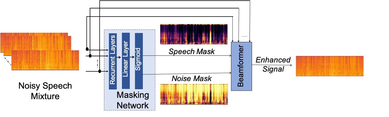
The neural beamforming method.

The beamforming process we used consists of the following stages:

• A neural network is trained to estimate speech and noise masks, given an input noisy signal. Since the training process is supervised, we create synthetic training data by adding CHiME-6 noises to VoxCeleb utterances (which are mostly clean). Note that a mask estimation network can only be trained on synthetic data, since there is no “ground truth” in case of real noisy data.

• The noisy input signal is fed into the neural network, and it predicts speech and noise masks. These masks are used to steer the MVDR/GEV beamformer, discussed above.

Although neural beamforming has shown much promise in recent years, we couldn’t get it to work better than the simple filter-and-sum beamforming, and so it was not used in our final submission.