Think about tasks such as machine translation (MT), automatic speech recognition (ASR), or handwriting recognition (HWR). While these appear very distinct, on abstraction they share the same pipeline wherein given an input signal, we are required to predict some text. The difference only lies in the form of the input signal - it is a piece of text, a sound wave, or a line image, in the case of MT, ASR, and HWR, respectively.
In all of these tasks, OOV words are a major source of nuisance. What is an OOV word? Simply put, these are those words in the test dataset which are not seen in the training data, and as such, not present in the vocabulary - hence the name “out of vocabulary”. Even if the training vocabulary is very large (in fact, the name Large Vocabulary ASR is very common), the test data may still have words which were never seen before, for instance, names of people, places, or organizations.
A crude way of dealing with such OOV words may be to simply predict a special token <UNK> whenever they are encountered. However, this would lead to severe information loss, especially when all new names are replaced by the special token. This is where subwords come into the picture.
Subwords are smaller units that comprise words. They may be a single character, or even entire words.
For example, suppose our training vocabulary consists of just 2 words {‘speech’,’processing’}. If our language model is trained on word-level, we would only be able to predict these 2 words, and nothing else. So while testing, if we are required to predict the phrase “he sings in a choir”, our model would fail miserably. However, if we had trained on a subword-level (say, character level), we have a non-zero chance of predicting the phrase since all the characters are seen in the training. This provides sufficient motivation for using subwords in these tasks.
Traditionally, in ASR, subwords have been modeled using information from phonemes (distinct sound units), such that a subword corresponds to a phoneme unit. The intuition is that at test time, any new word can only be formed using phonemes of the language. However, this requires considerable domain knowledge, and even still, variations in accent or speaker can greatly affect test-time performance.
In MT, subwords first came into limelight with this popular paper from Seinrich and Haddow at the University of Edinburgh. They used a simple but effective Byte Pair Encoding (BPE) based approach to identify subword units in the text. The summary of their method is as follows:
- Fix a vocabulary size V according to your total data size.
- Separate all the characters in all the words.
- Merge the most frequent bigram into one token and add it to the vocabulary.
- Perform V such merge operations to get the final vocabulary.
This simple method performs extremely well in practice, and the authors were able to get improvements of about 1.1 BLEU points on an English to German translation task.
I was recently working on an HWR task which required similar subword modeling for OOV word recognition, and the remainder of this article is about the methods used and their performance.
Towards a likelihood-based model
The first method we tried was the BPE-based approach, and it gave improvements on the word-error rate (WER) over the word-based model. However, BPE is constrained in the sense that it is a deterministic technique. Once you have fixed the training vocabulary, every string can only be segmented in a specific way. This may hint at a loss of modeling power, and so our first hypothesis is that a probabilistic segmentation technique may perform better.
On further investigation, I found a recent paper which proposes a technique known as “subword regularization” for MT. The method consists of two parts: vocabulary learning, and subword sampling.
Vocabulary learning
Similar to the BPE-based technique, we start with all the characters distinct in every word, and merge until we reach the desired vocabulary size V. However, while BPE used the metric of most frequent bigram, the Unigram SR method ranks all subwords according to the likelihood reduction on removing the subword from the vocabulary. The top 80% of these are retained and the rest are discarded. Once this phase is over, we can now obtain the likelihood of observing a subword sequence given any string (sentence).
Subword sampling
We choose the top-k segmentations based on the likelihood, and then model them as a multinomial distribution $P(x_i \vert X) = \frac{P(x_i)^{\alpha}}{\sum_l P(x_i)^{\alpha}}$, where $\alpha$ is a smoothing hyperparameter. A smaller $\alpha$ leads to a more uniform distribution, while a larger $\alpha$ leads to Viterbi sampling (i.e., selection of the best segmentation).
The idea behind this method is “regularization by noise”. This means that the algorithm is expected to generalize well since we are now training it with some added noise by selecting several different segmentation candidates for any word, and so the model sees a wider variety of subwords during training.
For implementation, we used Google’s sentencepiece library, which is also the official code of the paper linked above, and integrated it in our Kaldi-based pipeline (see here). While the method supposedly performed well in MT, we didn’t obtain the same performance improvements in the HWR task. A top-1 (deterministic) sampler gave similar results as BPE, but a top-5 sampler performed worse, which hinted that probabilstic sampling may not necessarily be the best suited option for our task.
For further analysis, I looked at the frequency of different subword lengths learned by the two methods for the same total vocabulary size.
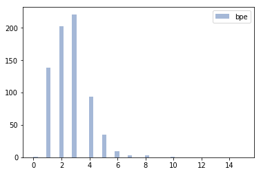
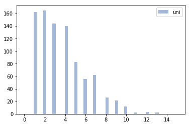
It turns out that the unigram method learns several “longer” subwords than BPE, which may give us some idea about the poorer performance. This suggested that if we somehow put a constraint on the lengths of the learned subwords while keeping the probabilistic sampling, we might get the best of both worlds.
Digression - The Morfessor tool
Readers familiar with linguistics (or morphology in particular) would have heard about (or used) the Morfessor tool, which provides an unsupervised technique for morpheme recognition. Morphemes, in a crude sense, are essentially subword units which are self-contained in meaning. Interestingly, the first Morfessor paper proposed a technique which is very similar to the likelihood-based subword modeling in the unigram SR paper (although the author does not seem to be aware of this). Additionally, they also proposed a minimum description length (MDL) based approach which added the subword lengths as a cost in the objective function, and therefore penalized longer subwords. Empirically, they found that the MDL technique outperformed the likelihood based method, and this further reinforced my belief that a subword length constraint would prove beneficial for the task.
LZW-based subword modeling
In an Interspeech 2005 paper, a new subword modeling algorithm was presented which supposedly correlated strongly with syllables of a language. The method is based on the popular LZW compression technique (which is also used in the Unix compress utility). In the context of strings, the LZW method finds a set of prefix-free substrings to encode the given string. The authors of the paper further used subword length tables to keep track of how many times each such subword was called during training, and thus ranked them within the tables. The test-time segmentation was determined by computing the average rank of all the segmentation candidates in this tree traversal.
In our implementation, we further integrated the probabilistic sampling method from the unigram SR, and used memoization to make the tree traversal computationally efficient. The implementation for learning and applying the model can be found here and here, respectively.
Perhaps the most critical segments of the implementation are the following:
def learn_subwords_from_word(word, tab_seqlen, tab_pos, max_subword_length):
    w = ""
    pos = 0
    for i,c in enumerate(word):
        if (i == len(word) - 1):
            pos = 2
        wc = w + c
        if (len(wc) > max_subword_length):
            wc = c

        if wc in tab_seqlen[len(wc)-1]:
            w = wc
            tab_seqlen[len(wc)-1][wc] += 1
        else:
            tab_seqlen[len(wc)-1][wc] = 1
            w = c
        if wc in tab_pos[pos]:
            w = wc
            tab_pos[pos][wc] += 1
            i -= 1
        else:
            tab_pos[pos][wc] = 1
            w = c
            pos = min(i,1)
def compute_segment_scores(word, tab_seqlen, tab_pos, scores):
    if (len(word) == 0):
        return ([])
    max_subword_length = len(tab_seqlen)
    seg_scores = []
    for i in range(max_subword_length):
        if(i < len(word)):
            subword = word[:i+1]
            if subword in tab_seqlen[i]:
                other_scores = []
                subword_score = float(tab_seqlen[i][subword][1]/(((i+1)**max_subword_length)*len(tab_seqlen[i])))
                if (word[i+1:] in scores):
                    other_scores = copy.deepcopy(scores[word[i+1:]])
                else:
                    other_scores = copy.deepcopy(compute_segment_scores(word[i+1:], tab_seqlen, tab_pos, scores))
                if (len(other_scores) == 0):
                    seg_scores.append(([subword],subword_score))
                else:
                    for j,segment in enumerate(other_scores):
                        other_scores[j] = ([subword]+segment[0],subword_score+segment[1])
                    seg_scores += other_scores
    seg_scores = sorted(seg_scores, key=lambda item: item[1])
    scores[word] = seg_scores
    return seg_scores
It may be noted here that the score of a segmentation candidate is calculated as the sum of the scores for all the subwords in that segmentation, where the score of subword $\sigma_w$ is defined as
\[\sigma_w = w \times \text{relative rank of subword in its table}\]Here, $w = \left(\frac{1}{\vert w\vert}\right)^{\max_w{\vert w\vert}}$. This score empirically gives subword lengths which correspond closely with the distribution of syllable lengths in English. It is a variation of the scoring scheme proposed in the original paper.
An analysis of the subword length frequencies obtained using this method reveals the following.
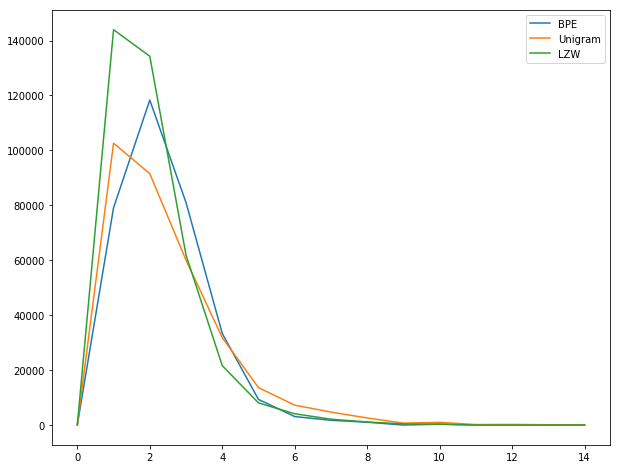
As expected, it produces more subwords of shorter lengths. A log-scale graph reveals further details about frequencies of longer subwords.
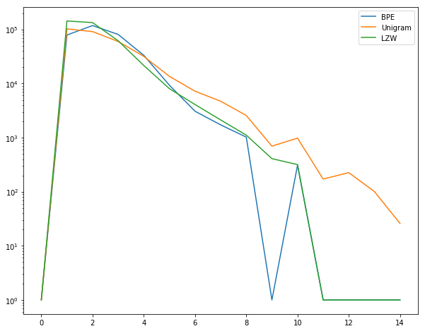
For higher lengths, LZW corresponds strongly with BPE, while unigram SR is nowhere close.
However, in the actual task, the method performs worse than both BPE and unigram, and this further strengthed my belief that probabilistic sampling, while useful for MT, does not quite fit in this particular HWR dataset.
Conclusion
While BPE seems like an ad-hoc technique for modeling subword units, it actually performs exceptionally well in practice. This, combined with its simplicity of implementation and low time complexity, makes it a great candidate for the task.
However, I believe that if a subword model were informed by the grapheme units (for HWR), as early techniques for ASR were informed by phonemes, it might perform well on the task. This seems like an interesting direction for exploration.